What is Logarithm
A logarithm is an inverse function of exponentiation. A simplified way of saying the same would be, that a logarithm is the opposite of an exponent. E.g.
The exponent form 2^3 = 8 can be written in its (opposite) logarithm form as \log_2 8 = 3
Let us describe the above mathematical forms in their simple English equivalents.
2^3 = 8, asks the question what will be the value if 2 grows 3 times? Answer is 8
\log_2 8 = 3, asks the question how many times will 2 have to grow to reach 8? The answer is 3 times
What is Natural Logarithm?
A natural logarithm is a special case of logarithm which has Euler’s constant (e) as its base. Mathematically Euler’s constant can be written as e^x. If we convert this into logarithmic form, we get the natural log.
e^x = a ==> \log_e a = x
The logarithm form is denoted as ln(a), which is called natural log.
Let us describe these mathematical forms in their simple English equivalent.
e^x = a , asks the question what will be the value if e grows x times ? Answer is a
ln(a) ==> \log_e a = x , asks the question how many times will e have to grow to reach a> Answer is x times.
Practical Application of Logarithm
Logarithms have practical applications in the following:
Scaling in Graphs
In graphs, logarithms are used for displaying a large range of values in compact space. For example, consider this covid death data plotted in both linear and log axis. The left side shows linear scale of deaths on Y-Axis. The right side graph shows logarithmic scale of deaths on Y-Axis. We have used logarithm to compact the size of the Y-Axis.
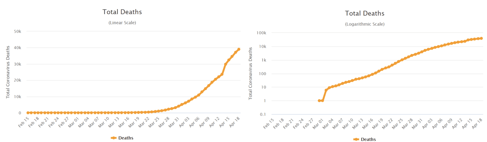
It is interesting to note that about 60% of the respondent in a recent survey by LSE did not understand what was being explained by a logarithmic graph. In another interesting article, Mordechai Rorvig explains the dynamics of log scale graphing and the cautions required in reading the logarithm axis.
Measurement scales
Logarithms are used in measurement scales where calculations require taking values over a large range into consideration. A few examples of measurement scales engaging logarithms are
Ritcher scale for earthquake monitoring
The Richter scale is logarithmic and uses a base of 10, meaning that whole-number jumps indicate a tenfold increase. In this case, the increase is in wave amplitude. That is, the wave amplitude in a level 6 earthquake is 10 times greater than in a level 5 earthquake, and the amplitude increases 100 times between a level 7 earthquake and a level 9 earthquake.
Google page rank algorithm
Google’s page rank algorithm shows the relative authority and traffic of a website on a scale between 0 -10. A higher number means higher traffic. The PageRank score is a logarithmic score. The actual calculation takes a lot of factors into account e.g. backlinks, referring domains, pr quality, authority score, etc. For this illustration, I have only taken traffic as an indicator. The two columns with log values calculate the rank with base 10 and 6 respectively. The main idea here is that we can use logarithms to represent a large-scale variation with a smaller number which makes intuitive sense for readers.
|
Domain |
Monthly visits
(similarweb.com) |
log10(x)=Pagerank |
log6(x)=Pagerank |
Estimated Google Pagerank
(checkpagerank.net) |
|
cnn.com |
524,000,000 |
8.7 |
11.2 |
9 |
|
latrobe.edu.au |
22,000,000 |
7.3 |
9.4 |
6 |
Growth & decay
Logarithmic growth is the inverse of exponential growth and is very slow. Exponential growth starts slowly and then speeds up. Logarithmic growth starts fast and then slows down.
The function of logarithmic growth describes a relationship where the result can be described as a log function of input
f(t)= A.Log(t) + B
The confusion between logarithmic growth and exponential growth can be explained by the fact that exponential growth curves may be straightened by plotting them using a logarithmic scale for the growth axis.
This article aims to summarise attributes available in any facebook campaign at the time of configuration. Having an overview of campaign attributes available is handy in understanding what can be analyzed,configured and managed within facebook campaigns. Depending on your role, you can go through the article to achieve the following objectives:
Data Analysts: If you are a data analyst, you can use the attributes below to understand what are your possible dimensions of analysis.
Data Scientists : If you are a data scientist, you can use the attributes to identify features for your data science model.
Campaign Managers : If you are a campaign manager, you can use the attributes as options available to configure,manage and optimise your campaign.
Facebook Campaign
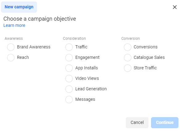
Facebook Ads Manager is used for creating campaigns. The first step in creating a campaign is to select its Objectives. Clicking on a Create Campaign button, opens selection choice for objective.
Campaign attribute summary
Attribute summary of campaign is given in the table below:
|
Category |
Campaign Objectives |
Description |
|
Awareness |
Brand Awareness |
Show your ads to people who are most likely to remember them. |
|
Reach |
Show your ads to the maximum number of people. |
|
Consideration |
Traffic |
Send people to a website, app or Facebook event, or let them tap to call you. |
|
Engagement |
Get more Page likes, event responses, or post reacts, comments or shares. |
|
App Installs |
Show your ad to people most likely to download and engage with your app. Learn more |
|
Video Views |
Show people video ads. |
|
Lead Generation |
Use forms, calls or chats to gather info from people interested in your business. Learn more |
|
Messages |
Show people ads that allow them to engage with you on Messenger, WhatsApp and Instagram. |
|
Conversions |
Conversions |
Show your ads to the people who are most likely to take action, such as buying something or calling you from your website. |
|
Catalogues Sales |
Use your target audience to show people ads with items from your catalogue. |
|
Store Traffic |
Show your ad to people most likely to visit your physical shops when they're near them. Learn more |
Facebook Bidding Strategies
Facebook Ad ecosystem is Auction based. Advertisers compete for ad space ( placement ). Facebook provides the following strategies to accomplish the Ad auctions.
|
Category |
Bid Strategy |
Description |
|
Spend-based |
Lowest Cost |
Get the most result for your budget |
|
|
Highest Value |
Spend your budget and focus on highest value purchases |
|
Goal-Based |
Cost Cap |
Strive to keep costs around the cost amount regardless of market conditions |
|
|
Minimum ROAS |
Budget Type |
|
Manual |
Bid Cap |
Manually control bids |
Facebook Budget
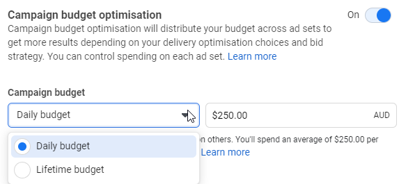
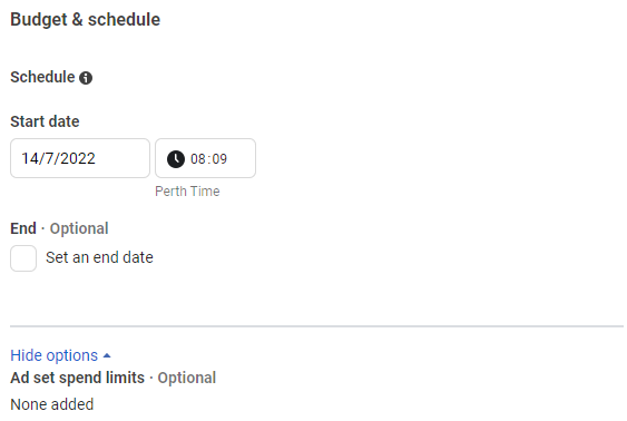
Budget is the total amount you want to spend for the campaign. Budget can be configured at two levels.
- Campaign Budget : Budget for entire campaign.
- Ad Set Budget : Budget for individual Ad Sets within campaigns.
Campaign Budget
Campaign budget applies to all Ad Sets within a campaign. It can be set on a daily basis or lifetime of campaign basis.
Ad Set Budget
Ad Set budget is defined at an Adset level. After you create a campaign, you can choose whether you want to create budget for Ad Set. It is optional. If it is not set, then campaign budget will determine Ad Set Budget.
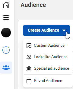
Facebook Audiences
Facebook supports few types of audiences.
- Core Audience: Defined from Adset panel, with limited options.
- Custom Audience: Defined from Audience Builder, with a lot more options than core audience.
- Look Alike Audience : Uses facebook’s algorithm to find new people similar to another audience.
- Special Ad Audience : Only available for users in special ads categories of credit, employment and housing ads.
You can create last 3 audiences from Audience manager.
Core Audience
Core Audeinces is defined from default adset. We can select from Location, Age, Gender, Demographic, interest, behavior and connections.
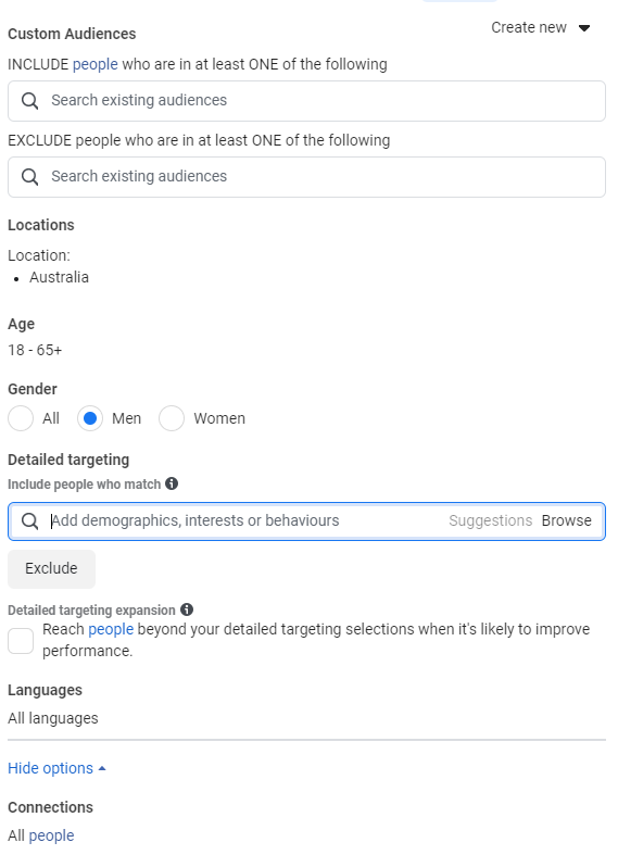
Custom Audience
Custom audiences provide a lot more attributes for selection. You can create custom audiences from audience manager or from the Ad set option
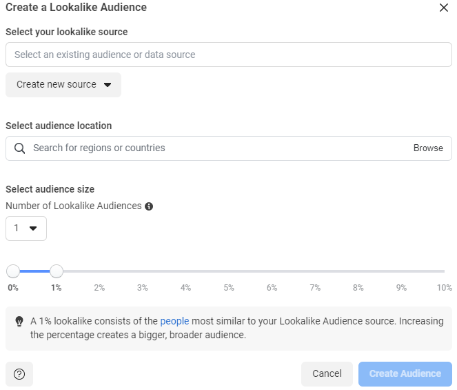
Lookalike Audience
A lookalike audience is built from an existing audience source. We provide the source, facebook find similar audiences. We can control the level of similarity ( or difference ) between source and target audience. For analysis purposes, three attributes of interest would be :
- Lookalike source
- Location
- Similarity Percentage.
Within facebook, creation of lookalike audience will be done from this screen.
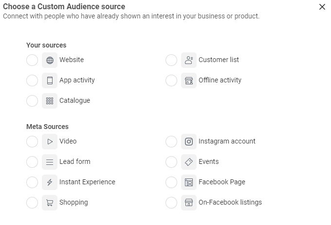
Audience attribute summary
Attribute summary of audiences is given in the table below:
|
Audience Type |
Category |
Attributes |
Description |
|
Core Audience |
|
|
Defined using default audience panel within the AdSet creation section. |
|
Custom Audience |
Your Sources |
Website |
Custom audiences which can be created in facebook from our own audience data or from facebook audience data. |
|
Customer List |
|
App Activity |
|
Offline Activity |
|
Catalogue |
|
Meta Sources |
Video |
|
Instagram Account |
|
Lead form |
|
Events |
|
Instant Experience |
|
Facebook Page |
|
Shopping |
|
On-Facebook Listings |
|
Lookalike Audiences |
Mixed |
Lookalike source |
Using machine learning algoritm to create audiences which have relatively similar attributes than original audiences. |
|
Location |
|
Similarity percentage |
|
Special Ad Audience |
Lookalike source |
Restricted for Credit, Employment or Housing |
|
Location |
|
Similarity percentage |
Facebook Placements
Placement is where our Ads show up. It is of significant importance in any campaign performance analysis. Same ad shown on top placement may have different efficiency as compared to a bottom placement.
There are two placement selection choices in facebook.
- Automatic placement : Facebook’s delivery system allocates your ad set’s budget across multiple placements. You do not have much control over it.
- Manual placement : You choose which placements you want your ad to be displayed on.
There are eight categories of placement in facebook, each comprising of several types of placements. Let us review all possible attributes in facebook placement.
Placements attribute summary
Mobile Devices & operating systems.
Within the Adset configuration, we can also choose which mobile devices and operating systems you want to target your ads on. If you are looking to analyse apple users(iOS) vs samsung users(Android), this will be your starting point. There are 4 options available at the time of writing.
Mobile Devices attribute summary
- All mobile devices
- Android devices only
- iOS devices only
- Feature phones only
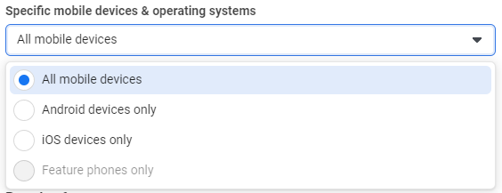
Another option available for mobile delivery is whether you want to display Ads, when audience is connected to wi-fi.

Optimization and Delivery
By selecting an optimisation method, you inform facebook on what does success mean for your campaign. Based on your “success criteria”, facebook’s machine learning algorithm can work to (optimise) tweak campaign parameters to get desired success results.
Optimisation attribute summary
Optimisation methods vary for each campaign objective. Here is a quick summary of what optimisation methods are available for each campaign type.
|
Category |
Campaign Objective |
Optimisation method |
Optimisation method description |
|
Awareness |
Brand Awareness |
Ad recall lift |
Facebook will serve your ads to maximise the total number of people who will remember seeing your ads. |
|
Reach |
Reach |
Facebook will serve your ads to the maximum number of people |
|
Impressions |
Facebook will deliver your ads to people as many times as possible |
|
Consideration |
Traffic |
Landing page views |
Facebook will deliver your ads to people who are more likely to click on your ad's link and load the website or Instant Experience. (Pixel) |
|
Link clicks |
Facebook will deliver your ads to the people most likely to click on them. |
|
Impressions |
Facebook will deliver your ads to people as many times as possible. |
|
Daily unique reach |
Facebook will deliver your ads to people up to once a day. |
|
|
|
|
Engagement |
Impressions |
Facebook will deliver your ads to people as
many times as possible. |
|
Post
Engagement |
Facebook will deliver your ads to the right
people to help you get the most likes, shares or comments on your post at the
lowest cost. |
|
Daily
unique reach |
Facebook will deliver your ads to people up
to once a day. |
|
Page
likes |
Facebook will deliver your ads to the right
people to help you get more Page likes at the lowest cost. |
|
Event
responses |
Facebook will deliver your ads to the right
people to help you get the most event interest at the lowest cost. |
|
App Installs |
App
Installs |
Facebook will deliver your ads to the people most
likely to install your app. |
|
Link
clicks |
Facebook willdeliver your ads to the people most
likely to install your app. |
|
App
Events |
Facebook will deliver your ads to the people most
likely to install your app. |
|
Value |
Facebook willdeliver your ads to the people most
likely to install your app. |
|
Video Views |
ThruPlay |
Facebook will deliver your ads to help you get the most completed video plays if the video is 15 seconds or shorter. For longer videos, this will optimise for people most likely to play at least 15 seconds. |
|
2-second continuous video views |
Facebook will deliver your ads to get the most video views of two continuous seconds or more. Most 2-second continuous video views will have at least 50% of the video pixels on screen. |
|
Lead Generation |
Leads |
We'll deliver your ads to the right people to help you get the most leads at the lowest cost. |
|
Conversion leads |
Facebook will deliver your ads to help you get leads that are most likely to convert. |
|
Messages |
Conversations |
Facebook will deliver your ads to people
most likely to have a conversation with you through messaging. |
|
Leads |
Facebook will deliver your ads to the right
people to help you get the most leads at the lowest cost. |
|
Link
clicks |
Facebook will deliver your ads to the people
most likely to click on them. |
|
Replies |
Facebook will deliver your ads to people
most likely to have a conversation with you through messages. |
|
Conversions |
Conversions |
Conversions |
Facebook will deliver your ads to the right
people to help you get the most website conversions. |
|
Conversations |
Facebook will deliver your ads to people
most likely to have a conversation with you through messaging. |
|
Link
clicks |
Facebook will deliver your ads to the people
most likely to click on them. |
|
Impressions |
Facebook will deliver your ads to people as
many times as possible. |
|
Daily
unique reach |
Facebook will deliver your ads to people up
to once a day. |
|
Catalogues Sales |
Value |
Facebook will deliver your ads to people to
maximise the total purchase value generated and get the highest return on ad
spend (ROAS). |
|
Conversion
events (suggested option) |
Facebook will deliver your ads to people
more likely to take action when they see a product from your catalogue. |
|
Link
clicks |
Facebook will deliver your ads to the people
most likely to click on them. |
|
Impressions |
Facebook will deliver your ads to people as
many times as possible. |
|
Store Traffic |
Daily
unique reach |
Facebook will deliver your ads to people up
to once a day. |
|
Store
visit |
Facebook will deliver your ads to people
more likely to visit your business locations. |
Exploring Google Analytics E-commerce Data.
We can explore machine learning capabilities of Google BigQuery by creating a classification model. The model will predict whether or not a new user is likely to purchase in future.
BigQuery ML supports following machine learning models.
A. Regression Models
1. Forecasting using linear regression
2. Classification using logistic regression
B. Classification Models
1. Deep Neural Networks
2. Boosted Decision Trees
3. AutoML Tables Models
4. Custom TensorFlow Models
E-commerce Conversion Rate.
#standardSQL
WITH visitors AS(
SELECT
COUNT(DISTINCT fullVisitorId) AS total_visitors
FROM `data-to-insights.ecommerce.web_analytics`
),
purchasers AS(
SELECT
COUNT(DISTINCT fullVisitorId) AS total_purchasers
FROM `data-to-insights.ecommerce.web_analytics`
WHERE totals.transactions IS NOT NULL
)
SELECT
total_visitors,
total_purchasers,
total_purchasers / total_visitors AS conversion_rate
FROM visitors, purchasers
The result will show us a conversion rate of 2.69%
| 1 |
741721
|
20015
|
0.026984540008979117
|
Top 5 selling products
SELECT
p.v2ProductName,
p.v2ProductCategory,
SUM(p.productQuantity) AS units_sold,
ROUND(SUM(p.localProductRevenue/1000000),2) AS revenue
FROM `data-to-insights.ecommerce.web_analytics`,
UNNEST(hits) AS h,
UNNEST(h.product) AS p
GROUP BY 1, 2
ORDER BY revenue DESC
LIMIT 5;
Result shows the following table
| 1 |
Nest® Learning Thermostat 3rd Gen-USA – Stainless Steel
|
Nest-USA
|
17651
|
870976.95
|
|
| 2 |
Nest® Cam Outdoor Security Camera – USA
|
Nest-USA
|
16930
|
684034.55
|
|
| 3 |
Nest® Cam Indoor Security Camera – USA
|
Nest-USA
|
14155
|
548104.47
|
|
| 4 |
Nest® Protect Smoke + CO White Wired Alarm-USA
|
Nest-USA
|
6394
|
178937.6
|
|
| 5 |
Nest® Protect Smoke + CO White Battery Alarm-USA
|
Nest-USA
|
6340
|
178572.4
|
Subsequent Visit Purchasers
# visitors who bought on a return visit (could have bought on first as well
WITH all_visitor_stats AS (
SELECT
fullvisitorid, # 741,721 unique visitors
IF(COUNTIF(totals.transactions > 0 AND totals.newVisits IS NULL) > 0, 1, 0) AS will_buy_on_return_visit
FROM `data-to-insights.ecommerce.web_analytics`
GROUP BY fullvisitorid
)
SELECT
COUNT(DISTINCT fullvisitorid) AS total_visitors,
will_buy_on_return_visit
FROM all_visitor_stats
GROUP BY will_buy_on_return_visit
About 1.6% of total visitors will return and purchase from the website.
Feature Engineering.
We will build two models by selecting different features and compare their performance
Feature Set 1 for First model
We will use two input fields for the classification model.
Bounces given by field totals.bounces. A visit is counted as a bounce if a visitor does not engage in any activity on the website after opening the page and leaves.
Time on site given by field totals.timeOnSite. This field determins total time visitor was on our website.
SELECT
* EXCEPT(fullVisitorId)
FROM
# features
(SELECT
fullVisitorId,
IFNULL(totals.bounces, 0) AS bounces,
IFNULL(totals.timeOnSite, 0) AS time_on_site
FROM
`data-to-insights.ecommerce.web_analytics`
WHERE
totals.newVisits = 1)
JOIN
(SELECT
fullvisitorid,
IF(COUNTIF(totals.transactions > 0 AND totals.newVisits IS NULL) > 0, 1, 0) AS will_buy_on_return_visit
FROM
`data-to-insights.ecommerce.web_analytics`
GROUP BY fullvisitorid)
USING (fullVisitorId)
ORDER BY time_on_site DESC
LIMIT 10;
We get the following output
| 1 |
0
|
15047
|
0
|
|
| 2 |
0
|
12136
|
0
|
|
| 3 |
0
|
11201
|
0
|
|
| 4 |
0
|
10046
|
0
|
|
| 5 |
0
|
9974
|
0
|
|
| 6 |
0
|
9564
|
0
|
|
| 7 |
0
|
9520
|
0
|
|
| 8 |
0
|
9275
|
1
|
|
| 9 |
0
|
9138
|
0
|
|
| 10 |
0
|
8872
|
0
|
Feature set 2 for second model:
For our second model, we will use entirely different set of features.
- Visitors Journey progress given by field hits.eCommerceAction.action_type. It denotes progress with integer field where 6 = completed purchase
- Traffic source by trafficsource.source and trafficsource.medium
- Device category given by field device.deviceCategory
- Country given by field geoNetwork.country
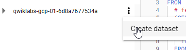
Creating model in BigQuery.
Creating dataset for the model
Before creating a model in BigQuery, we will create a BigQuery dataset to store the models.
Selecting Model type
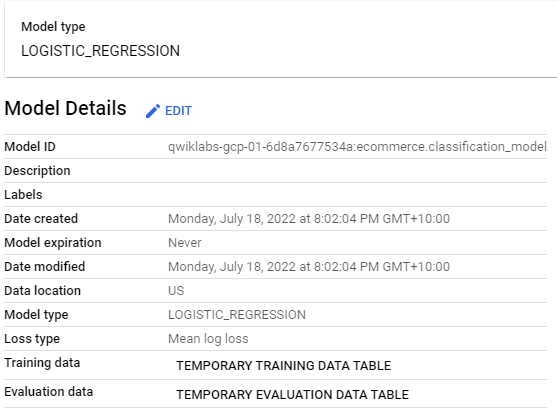
Since we are predicting a binary class ( whether user will buy or not) , we will go with classification using logistic regression.
Classification using Logistic Regression Model:
CREATE OR REPLACE MODEL `ecommerce.classification_model`
OPTIONS
(
model_type='logistic_reg',
labels = ['will_buy_on_return_visit']
)
AS
#standardSQL
SELECT
* EXCEPT(fullVisitorId)
FROM
# features
(SELECT
fullVisitorId,
IFNULL(totals.bounces, 0) AS bounces,
IFNULL(totals.timeOnSite, 0) AS time_on_site
FROM
`data-to-insights.ecommerce.web_analytics`
WHERE
totals.newVisits = 1
AND date BETWEEN '20160801' AND '20170430') # train on first 9 months
JOIN
(SELECT
fullvisitorid,
IF(COUNTIF(totals.transactions > 0 AND totals.newVisits IS NULL) > 0, 1, 0) AS will_buy_on_return_visit
FROM
`data-to-insights.ecommerce.web_analytics`
GROUP BY fullvisitorid)
USING (fullVisitorId)
;
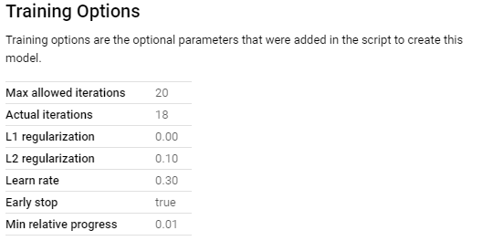
We can now create model in our newly created ecommerce table. It will show the following information.
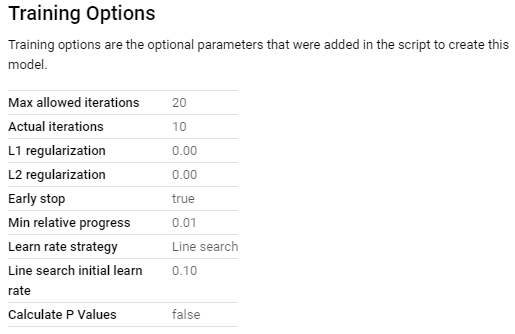
Classification using Logistic Regression with Feature Set 2
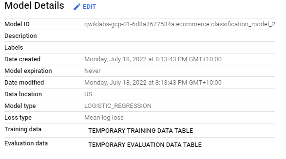
CREATE OR REPLACE MODEL `ecommerce.classification_model_2`
OPTIONS
(model_type='logistic_reg', labels = ['will_buy_on_return_visit']) AS
WITH all_visitor_stats AS (
SELECT
fullvisitorid,
IF(COUNTIF(totals.transactions > 0 AND totals.newVisits IS NULL) > 0, 1, 0) AS will_buy_on_return_visit
FROM `data-to-insights.ecommerce.web_analytics`
GROUP BY fullvisitorid
)
# add in new features
SELECT * EXCEPT(unique_session_id) FROM (
SELECT
CONCAT(fullvisitorid, CAST(visitId AS STRING)) AS unique_session_id,
# labels
will_buy_on_return_visit,
MAX(CAST(h.eCommerceAction.action_type AS INT64)) AS latest_ecommerce_progress,
# behavior on the site
IFNULL(totals.bounces, 0) AS bounces,
IFNULL(totals.timeOnSite, 0) AS time_on_site,
totals.pageviews,
# where the visitor came from
trafficSource.source,
trafficSource.medium,
channelGrouping,
# mobile or desktop
device.deviceCategory,
# geographic
IFNULL(geoNetwork.country, "") AS country
FROM `data-to-insights.ecommerce.web_analytics`,
UNNEST(hits) AS h
JOIN all_visitor_stats USING(fullvisitorid)
WHERE 1=1
# only predict for new visits
AND totals.newVisits = 1
AND date BETWEEN '20160801' AND '20170430' # train 9 months
GROUP BY
unique_session_id,
will_buy_on_return_visit,
bounces,
time_on_site,
totals.pageviews,
trafficSource.source,
trafficSource.medium,
channelGrouping,
device.deviceCategory,
country
);
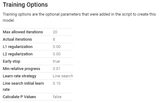
Classification using XGBoost with Feature Set 2
We can use the feature set used in the second model to create another model, however, this time using XGBoost.
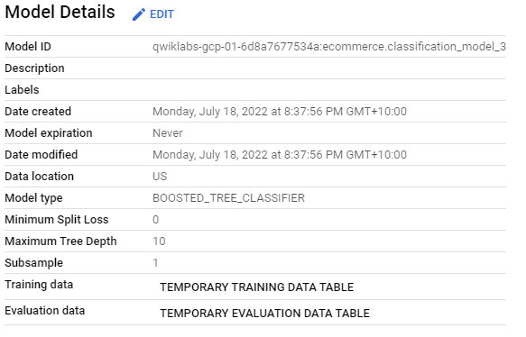
CREATE OR REPLACE MODEL `ecommerce.classification_model_3`
OPTIONS
(model_type='BOOSTED_TREE_CLASSIFIER' , l2_reg = 0.1, num_parallel_tree = 8, max_tree_depth = 10,
labels = ['will_buy_on_return_visit']) AS
WITH all_visitor_stats AS (
SELECT
fullvisitorid,
IF(COUNTIF(totals.transactions > 0 AND totals.newVisits IS NULL) > 0, 1, 0) AS will_buy_on_return_visit
FROM `data-to-insights.ecommerce.web_analytics`
GROUP BY fullvisitorid
)
# add in new features
SELECT * EXCEPT(unique_session_id) FROM (
SELECT
CONCAT(fullvisitorid, CAST(visitId AS STRING)) AS unique_session_id,
# labels
will_buy_on_return_visit,
MAX(CAST(h.eCommerceAction.action_type AS INT64)) AS latest_ecommerce_progress,
# behavior on the site
IFNULL(totals.bounces, 0) AS bounces,
IFNULL(totals.timeOnSite, 0) AS time_on_site,
totals.pageviews,
# where the visitor came from
trafficSource.source,
trafficSource.medium,
channelGrouping,
# mobile or desktop
device.deviceCategory,
# geographic
IFNULL(geoNetwork.country, "") AS country
FROM `data-to-insights.ecommerce.web_analytics`,
UNNEST(hits) AS h
JOIN all_visitor_stats USING(fullvisitorid)
WHERE 1=1
# only predict for new visits
AND totals.newVisits = 1
AND date BETWEEN '20160801' AND '20170430' # train 9 months
GROUP BY
unique_session_id,
will_buy_on_return_visit,
bounces,
time_on_site,
totals.pageviews,
trafficSource.source,
trafficSource.medium,
channelGrouping,
device.deviceCategory,
country
);
Evaluating performance of trained model.
We can evaluate classification models using a few metrics. Let us go with the basics.
ROC for logistic regression model with Feature Set 1
When we create a logistic regression classification model, we can access roc_auc field in BigQuery to automatically draw an ROC curve.
SELECT
roc_auc,
CASE
WHEN roc_auc > .9 THEN 'good'
WHEN roc_auc > .8 THEN 'fair'
WHEN roc_auc > .7 THEN 'not great'
ELSE 'poor' END AS model_quality
FROM
ML.EVALUATE(MODEL ecommerce.classification_model, (
SELECT
* EXCEPT(fullVisitorId)
FROM
# features
(SELECT
fullVisitorId,
IFNULL(totals.bounces, 0) AS bounces,
IFNULL(totals.timeOnSite, 0) AS time_on_site
FROM
`data-to-insights.ecommerce.web_analytics`
WHERE
totals.newVisits = 1
AND date BETWEEN '20170501' AND '20170630') # eval on 2 months
JOIN
(SELECT
fullvisitorid,
IF(COUNTIF(totals.transactions > 0 AND totals.newVisits IS NULL) > 0, 1, 0) AS will_buy_on_return_visit
FROM
`data-to-insights.ecommerce.web_analytics`
GROUP BY fullvisitorid)
USING (fullVisitorId)
));
The output we get is :
| 1 |
0.72386313686313686
|
not great
|
ROC for logistic regression model with Feature Set 2
#standardSQL
SELECT
roc_auc,
CASE
WHEN roc_auc > .9 THEN 'good'
WHEN roc_auc > .8 THEN 'fair'
WHEN roc_auc > .7 THEN 'not great'
ELSE 'poor' END AS model_quality
FROM
ML.EVALUATE(MODEL ecommerce.classification_model_2, (
WITH all_visitor_stats AS (
SELECT
fullvisitorid,
IF(COUNTIF(totals.transactions > 0 AND totals.newVisits IS NULL) > 0, 1, 0) AS will_buy_on_return_visit
FROM `data-to-insights.ecommerce.web_analytics`
GROUP BY fullvisitorid
)
# add in new features
SELECT * EXCEPT(unique_session_id) FROM (
SELECT
CONCAT(fullvisitorid, CAST(visitId AS STRING)) AS unique_session_id,
# labels
will_buy_on_return_visit,
MAX(CAST(h.eCommerceAction.action_type AS INT64)) AS latest_ecommerce_progress,
# behavior on the site
IFNULL(totals.bounces, 0) AS bounces,
IFNULL(totals.timeOnSite, 0) AS time_on_site,
totals.pageviews,
# where the visitor came from
trafficSource.source,
trafficSource.medium,
channelGrouping,
# mobile or desktop
device.deviceCategory,
# geographic
IFNULL(geoNetwork.country, "") AS country
FROM `data-to-insights.ecommerce.web_analytics`,
UNNEST(hits) AS h
JOIN all_visitor_stats USING(fullvisitorid)
WHERE 1=1
# only predict for new visits
AND totals.newVisits = 1
AND date BETWEEN '20170501' AND '20170630' # eval 2 months
GROUP BY
unique_session_id,
will_buy_on_return_visit,
bounces,
time_on_site,
totals.pageviews,
trafficSource.source,
trafficSource.medium,
channelGrouping,
device.deviceCategory,
country
)
));
The result we get this time are :
| 1 |
0.90948851148851151
|
good
|
ROC for XGBoost Classifier with feature set 2:
#standardSQL
SELECT
roc_auc,
CASE
WHEN roc_auc > .9 THEN 'good'
WHEN roc_auc > .8 THEN 'fair'
WHEN roc_auc > .7 THEN 'not great'
ELSE 'poor' END AS model_quality
FROM
ML.EVALUATE(MODEL ecommerce.classification_model_3, (
WITH all_visitor_stats AS (
SELECT
fullvisitorid,
IF(COUNTIF(totals.transactions > 0 AND totals.newVisits IS NULL) > 0, 1, 0) AS will_buy_on_return_visit
FROM `data-to-insights.ecommerce.web_analytics`
GROUP BY fullvisitorid
)
# add in new features
SELECT * EXCEPT(unique_session_id) FROM (
SELECT
CONCAT(fullvisitorid, CAST(visitId AS STRING)) AS unique_session_id,
# labels
will_buy_on_return_visit,
MAX(CAST(h.eCommerceAction.action_type AS INT64)) AS latest_ecommerce_progress,
# behavior on the site
IFNULL(totals.bounces, 0) AS bounces,
IFNULL(totals.timeOnSite, 0) AS time_on_site,
totals.pageviews,
# where the visitor came from
trafficSource.source,
trafficSource.medium,
channelGrouping,
# mobile or desktop
device.deviceCategory,
# geographic
IFNULL(geoNetwork.country, "") AS country
FROM `data-to-insights.ecommerce.web_analytics`,
UNNEST(hits) AS h
JOIN all_visitor_stats USING(fullvisitorid)
WHERE 1=1
# only predict for new visits
AND totals.newVisits = 1
AND date BETWEEN '20170501' AND '20170630' # eval 2 months
GROUP BY
unique_session_id,
will_buy_on_return_visit,
bounces,
time_on_site,
totals.pageviews,
trafficSource.source,
trafficSource.medium,
channelGrouping,
device.deviceCategory,
country
)
));/* Your code... */
Our roc_auc metric has declined slightly ( by .02).
Making Predictions
Lastly, we can predict using our model which new visitors will come back and purchase.
BigQuery ML uses ml.PREDICT() function to make a prediction.
Our total dataset is 12 months. We are making prediction for only last 1 month.
Prediction with logistic regression model
We will use our logistic regression model to make predictions first.
SELECT
*
FROM
ml.PREDICT(MODEL `ecommerce.classification_model_2`,
(
WITH all_visitor_stats AS (
SELECT
fullvisitorid,
IF(COUNTIF(totals.transactions > 0 AND totals.newVisits IS NULL) > 0, 1, 0) AS will_buy_on_return_visit
FROM `data-to-insights.ecommerce.web_analytics`
GROUP BY fullvisitorid
)
SELECT
CONCAT(fullvisitorid, '-',CAST(visitId AS STRING)) AS unique_session_id,
# labels
will_buy_on_return_visit,
MAX(CAST(h.eCommerceAction.action_type AS INT64)) AS latest_ecommerce_progress,
# behavior on the site
IFNULL(totals.bounces, 0) AS bounces,
IFNULL(totals.timeOnSite, 0) AS time_on_site,
totals.pageviews,
# where the visitor came from
trafficSource.source,
trafficSource.medium,
channelGrouping,
# mobile or desktop
device.deviceCategory,
# geographic
IFNULL(geoNetwork.country, "") AS country
FROM `data-to-insights.ecommerce.web_analytics`,
UNNEST(hits) AS h
JOIN all_visitor_stats USING(fullvisitorid)
WHERE
# only predict for new visits
totals.newVisits = 1
AND date BETWEEN '20170701' AND '20170801' # test 1 month
GROUP BY
unique_session_id,
will_buy_on_return_visit,
bounces,
time_on_site,
totals.pageviews,
trafficSource.source,
trafficSource.medium,
channelGrouping,
device.deviceCategory,
country
)
)
ORDER BY
predicted_will_buy_on_return_visit DESC;
The output will be :
Models prediction : predicted_will_buy_on_return_visit ( 1=yes)
Models confidence : predicted_will_buy_on_return_visit_probs.prob
|
| 1 |
1
|
1
|
0.56384838909667623
|
5584156807534326199-1499456348
|
0
|
6
|
0
|
571
|
24
|
gdeals.googleplex.com
|
referral
|
Referral
|
desktop
|
United States
|
|
|
|
0
|
0.43615161090332377
|
|
|
|
|
|
|
|
|
|
|
|
|
| 2 |
1
|
1
|
0.53345977038719161
|
0608643970260729792-1499785056
|
1
|
6
|
0
|
620
|
14
|
gdeals.googleplex.com
|
referral
|
Referral
|
desktop
|
United States
|
|
|
|
0
|
0.46654022961280839
|
|
|
|
|
|
|
|
|
|
|
|
|
| 3 |
1
|
1
|
0.56460044526931086
|
5177128356817703126-1500354345
|
0
|
6
|
0
|
397
|
18
|
sites.google.com
|
referral
|
Referral
|
desktop
|
United States
|
Predictions with XGBoost model
SELECT
*
FROM
ml.PREDICT(MODEL `ecommerce.classification_model_3`,
(
WITH all_visitor_stats AS (
SELECT
fullvisitorid,
IF(COUNTIF(totals.transactions > 0 AND totals.newVisits IS NULL) > 0, 1, 0) AS will_buy_on_return_visit
FROM `data-to-insights.ecommerce.web_analytics`
GROUP BY fullvisitorid
)
SELECT
CONCAT(fullvisitorid, '-',CAST(visitId AS STRING)) AS unique_session_id,
# labels
will_buy_on_return_visit,
MAX(CAST(h.eCommerceAction.action_type AS INT64)) AS latest_ecommerce_progress,
# behavior on the site
IFNULL(totals.bounces, 0) AS bounces,
IFNULL(totals.timeOnSite, 0) AS time_on_site,
totals.pageviews,
# where the visitor came from
trafficSource.source,
trafficSource.medium,
channelGrouping,
# mobile or desktop
device.deviceCategory,
# geographic
IFNULL(geoNetwork.country, "") AS country
FROM `data-to-insights.ecommerce.web_analytics`,
UNNEST(hits) AS h
JOIN all_visitor_stats USING(fullvisitorid)
WHERE
# only predict for new visits
totals.newVisits = 1
AND date BETWEEN '20170701' AND '20170801' # test 1 month
GROUP BY
unique_session_id,
will_buy_on_return_visit,
bounces,
time_on_site,
totals.pageviews,
trafficSource.source,
trafficSource.medium,
channelGrouping,
device.deviceCategory,
country
)
)
ORDER BY
predicted_will_buy_on_return_visit DESC;
|
| 1 |
1
|
1
|
0.52540105581283569
|
8015915032010696677-1500581774
|
1
|
5
|
0
|
1198
|
16
|
sites.google.com
|
referral
|
Referral
|
desktop
|
United States
|
|
|
|
0
|
0.47459891438484192
|
|
|
|
|
|
|
|
|
|
|
|
|
| 2 |
1
|
1
|
0.52540105581283569
|
8168421017407336619-1500948344
|
1
|
5
|
0
|
1043
|
19
|
sites.google.com
|
referral
|
Referral
|
desktop
|
United States
|
|
|
|
0
|
0.47459891438484192
|
|
|
|
|
|
|
|
|
|
|
|
|
| 3 |
1
|
1
|
0.52540105581283569
|
8860823110638301167-1499466860
|
0
|
5
|
0
|
1176
|
17
|
sites.google.com
|
referral
|
Referral
|
desktop
|
United States
|
|
|
|
0
|
0.47459891438484192
|
|
|
|
|
|
|
|
|
|
|
|
|
| 4 |
1
|
1
|
0.547279417514801
|
1860094959713788549-1499748085
|
0
|
3
|
0
|
1084
|
22
|
mall.googleplex.com
|
referral
|
Referral
|
desktop
|
Canada
|
|
|
|
0
|
0.45272055268287659
|
|
|
|
|
|
|
|
|
|
|
Reference : https://www.coursera.org/learn/gcp-big-data-ml-fundamentals
self-notes
Leadership is talked quite often in modern day work places. What is meant by leadership is quite often reliant on speaker’s mental model of it. There is a high likelyhood that speaker(or the leader) may not have a structured mental model for what she means by leadership. In addition, the listener may have an entirely different understanding of leadership. The following leadership models summarize characteristic of a few leadership models and attempts to review how leadership models have evolved over time.
Heroic Leadership
Standard mode of thinking in individualistic culture revolves around the pattern of thinking where Leader is a hero and Saviour. A superman who saves the day.
| Theory |
Theme |
Contributing theorists |
Notes to self |
| Heroic Leadership |
Leader is born, not made. Leader possesses extra ordinary capabilities with which she can perform wonders which others cannot. |
Thomas Carlyle in 1840 originally phrased the term, Plato, Lao-tzu, Aristotle , Machiavelli have been contributing over time to this pattern of thinking. |
This theory is still dominant mode of thinking in workplace today. Recent HBR article tries to identify a few of its caveats here. |
Charismatic Leadership
Slightly modified version of the heroic leader. Charismatic leader may have inborn traits, but they also cquires the skills like charisma, integrity, motivation etc.
In the words of Riggio:
C”harismatic leaders are essentially very skilled communicators – individuals who are both verbally eloquent, but also able to communicate to followers on a deep, emptional level. They are able to articulate a compelling or captivating vision and are able to arouse strong emotions in followers.”
| Theory |
Theme |
Contributing theorists |
Notes to self |
| Charismatic Leader |
Leaders can acquire certain traits, which will help them in achieving desired objectives. |
Several |
This theory appeals because traits and characteristic are to some degree responsible for goal achievement e.g., for team building one would get a lot of help from integrity and conscientiousness. |
Behavioural Leadership
Trait theory ignored the context around leadership success. Behavioural theory built upon internal traits and said that external behaviors(supported by traits) of leaders contribute to the success.
| Theory |
Theme |
Contributing theorists |
Notes to self |
| Behavioural Leadership |
Traits are not always consistent. Therefore, external behaviour of leaders is determinant of success. Traits can be indicative of what behaviour to expect. But the actual consistency in behaviour determines success |
Katz, Maccoby, Gurin and Floor(1951), Stogdill and Coons(1957). |
Feels contributary to success. Consistency is the key and helps in achieving trust of the team. |
Contingent Leadership
Contingent theory ( 1967-1990) took into account contextual variable. Leader could have the best traits (trait theory), she could exhibit them in her behavior consistently(behavioral theory), however, the external factors had been missing in accounting for leadership success. Contingency theory takes into account people, situational, organizational and enviornmental factors.
Three of the most notable theories of this era were
1. Fiedler’s Contingency Theory,
2. House’s Path-Goal Theory,
3. Vroom and Yetton’s Normative Theory of Decision Making
Fiedler identified three managerial components:
- Leader-member relations
- Task structures
- Position power.
some contexts favoured leaders who were task-oriented and some favoured those who were relationship oriented.
| Theory |
Theme |
Contributing theorists |
Notes to self |
| Contingent Leadership |
No single style of leadership is universal. It all depends on the context.
(Traits + Behaviours) + context |
Fiedler(1967,1971),
Hershey & Blanchard(1969) |
Smaller organisation are often driven by task based leaders, larger organisation have influence power arranged in relationships. |
Servant Leaderhip
Originally coined in 1970 by Robert Greenleaf, servant leadership is linked to ethics, virtues and morality. Its origin go back through history with people such as confucius, Lao-tzu, Moses and Jesus Christ as examples of servant leader.
Spears identifies 10 characteristics of servant leaders:
- Receptive listening.
- Empathy.
- Healing : Recognizing they have opportunities to make themselves and others whole.
- Self Awareness.
- Persuation: Convincing over coersion.
- Conceptualisation: Nurturing the ability to envision greater possibilities.
- Foresight : Intuititvely learning lessons from past.
- Stewardship : Comitted first and foremost to serving the needs of the others.
- Commitment : to growth of people in personal, professional and spiritual realms.
- Building community: identifies means of building communities among individuals working within organizations.
This is my favourite theory because of its inherent beauty and contradictions in its implementation. It is beautiful because it is characterised by trust and respect between leaders and followers. It is despicable because of the practical lip service it gets in organization.It is truly difficult to embrace.
Now a days(2022) it is exhbited by inverting organogram, showing CEO at the bottom and employee at the top. I am always amused by CEO’s and top leaders inverting the hirearchy in an organogram and then “asking ( somewhat ordering) ” the followers to lead by “following” the new-found diagram of inverted hirearchy.
My sentiments are echoed in Robert Greenleaf’s questions (1970 ):
“The best test and difficult to administer is: do those served grow as persons; do they, while being served, become healthier, wiser, freer, more autonomous, more likely themselves to become servants? And what is the effect on the least privileged in society; will they benefit, or, at least, will they not be further deprived?”
| Theory |
Theme |
Contributing theorists |
Notes to self |
| Servant Leadership |
Leader serve the followers.
High quality relationship are characterised by trust and respect between leader and follower. Low quality relationship are characterised by transactional and contractual obligation |
Robert Greenleaf(1970),Graen & Uhl-Bien (1995), Gerstner & Day (1997), Nahrgang & Morgeson(2007) |
Theoretically wonderful, practically contradictory. Can a follower change strategy set out by leader? |
Transformational Leadership
In a rapidly changing world, transformational leadership model seeks adaptation to change from the leader.In change adaptation, It focuses on getting commitment from the follower rather than compliance,. A tranformational leadership model proposes a symbiotic relationship in contrast to a transactional relationship . A mutual simulation converts followers into leaders and leaders into moral agents. James MacGregor Burn’s work Leadership (1987) introduced this concept. James first termed the idea of ‘Transformational leadership’ as a balanced dynamic between leaders and followers predicated upon social influence, rather than power. It looked toward fulfillment of aspirational needs of people.
Bernard Bass ( influenced by James M.) detailed the structure of transformational leadership to include :
- Idealised behaviours : Walking the talk
- Inspirational motivation : Offering compelling vision .
- Intellectual simulation: Challenge followers to be innovative and creative .
- Individualized consideration : Ability of the leader to demonstrate genuine concern for needs and feelings of follower.
| Theory |
Theme |
Contributing theorists |
Notes to self |
| Transformational Leadership |
Leader-follower symbiosis for achieving common good. |
James Macgregor Burn (1987), Bernard & Bass (1985,1998) |
Heavy leaning on the idealistic side of the world. Asks a lot of leader, e.g. leader should be able to inspire motivation and intellectually simulate the follower. These 2 tasks in themselves are too uphill for mere mortals. |
System Leadership
System leadership recognises that collaboration is essential to solve wicked problems (Heifetz,Kani, and Kramer, 2004). Leaders in system leadership model sacrifice their ego for common good. They move from individual to collaborative responsibility. Reactivity is replaced pro-active collaboration. Leaders collaborate with followers to achieve a shared vision. Power distribution in the organisation is decentralized. Hirearchy has its foundation in mutual trust rather than vertical organogram.
| Theory |
Theme |
Contributing theorists |
Notes to self |
| System Leadership |
Decentralized power, mutual trust, and letting go of a leader’s ego for achieving shared vision |
Senge, Hamilton, and Kania (2015), Jim Collins, Fredric Laloux (2014) |
Especially in a knowledge-based economy, this model serves well. It solves the complexity of interconnected systems. It also nourishes individual autonomy and individual ideation while keeping focus on common goals. |
References :
Gene Early, A short history of leadership theories.
EdX, University of Queensland, Becoming an effective leader