Data Build Tool ( DBT ) offers functionalities for testing our data models to ensure their reliability and accuracy. DBT tests help in achieveing these objectives .
Overall, dbt testing helps achieve these objectives:
Improved Data Quality: By catching errors and inconsistencies early on, we prevent issues from propagating downstream to reports and dashboards.
Reliable Data Pipelines: Tests ensure that our data transformations work as expected, reducing the risk of regressions when code is modified.
Stronger Data Culture: A focus on testing instills a culture of data quality within organization.
This article is a continuation of previous hands-on implementation of DBT model. DIn this article, we will explore the concept of tests in DBT and how we can implement the tests.
Data Build Tool (DBT) provides a comprehensive test framework to ensure data quality and reliability. Here’s a summary of tests that dbt supports.
Test Type
Subtype
Description
Usage
Implementation method
Generic Tests
Built-in
Pre-built or out-of-the-box tests for common data issues such as uniqueness, not-null, and referential integrity.
unique, not_null, relationships,accepted_values
schema.yml using tests: key under model/column
Custom Generic Tests
Custom tests written by users that can be applied to any column or model, similar to built-in tests but with custom logic.
Custom reusable tests with user-defined SQL logic.
1. Dbt automatically picks up from tests/generic/test_name.sql starting with {% tests %} . 2. Schema.yml by defining tests in .sql file and applying in schema.yml 3.macros: Historically, this wa the only place they could be defined.
Singular Tests
Designed to validate a single condition and are not intended to be reusable e.g. check if total sales reported in a period matches the sum of individual sales record.
Custom SQL conditions specific to a model or field.
Dbt automatically picks up test from tests/test_name.sql
Source Freshness Tests
Tests that check the timeliness of the data in your sources by comparing the current timestamp with the last updated timestamp.
dbt source freshness to monitor data update intervals.
Schema.yml using freshness: key under source/table
DBT testing framework
Implementing Built-In Tests
We will begin by writing generic tests. As we saw in the table above there are two types, Built-in and Custom. We will begin with a built-in test.
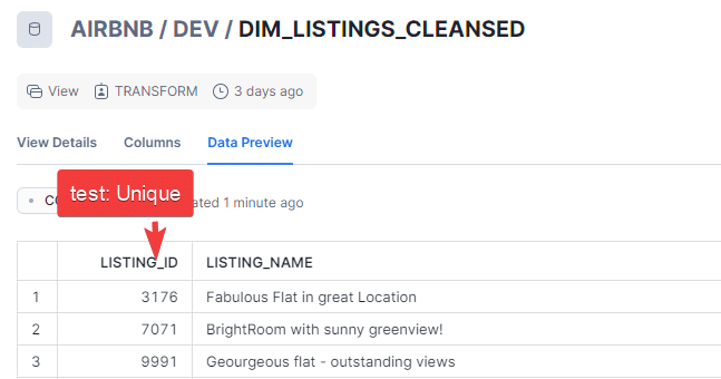
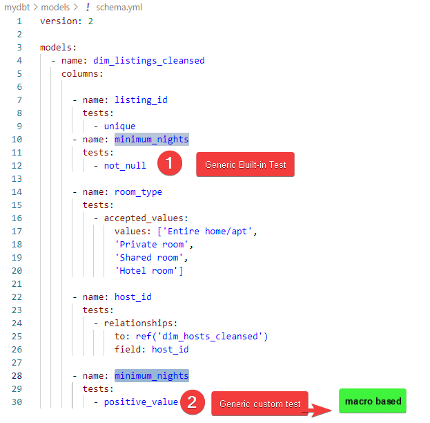
Built-in Tests 1.Unique :
We will explore this test with our model DEV.DIM_LISTING_CLEANSED.The objective is to make sure that all values in the column LISTING_ID are unique.
To implement tests we will create a new file schema.yml and define our tests in it.
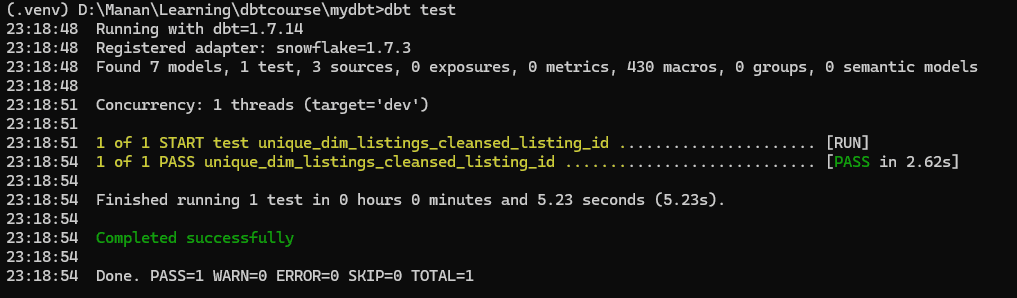
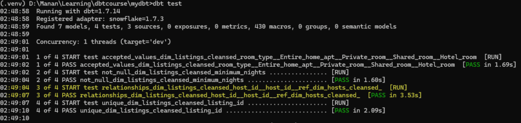
As we now run dbt test command in terminal, we will see the test execute and pass
Built-in Test 2.not_null
In the not_null example, we do not want any of the values in minimum nights column to be null. We will add another column name and test under the same hierarchy.
      - name: minimum_nights
        tests:
          - not_null
Now, when we execute dbt test, we will see another test added
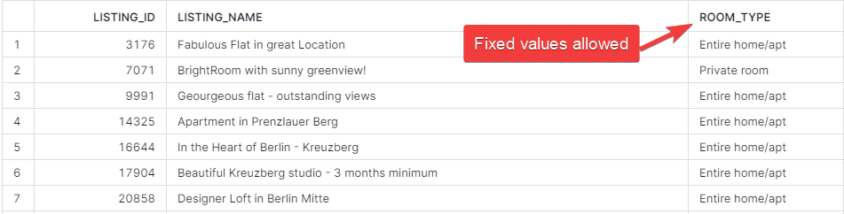
Built-in Test 3. accepted_values
In the accepted_values test, we will ensure that the column ROOM_TYPE in DEV.DIM_LISTING_CLEANSED can have preselected values only.
To add that test, we use the following entry in our source.yml file under model dim_listings_cleansed.
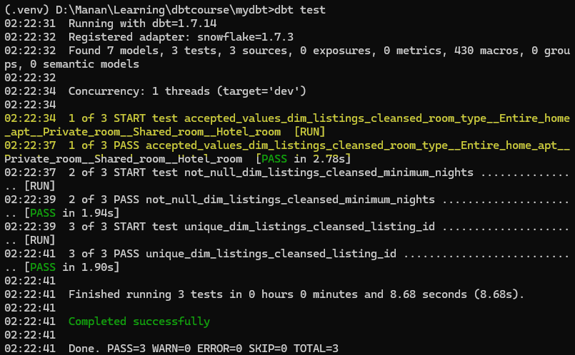
Now when we run dbt test, we can see another test executed which will check whether the column has only predetermined values as specificed in accepted_values or not.
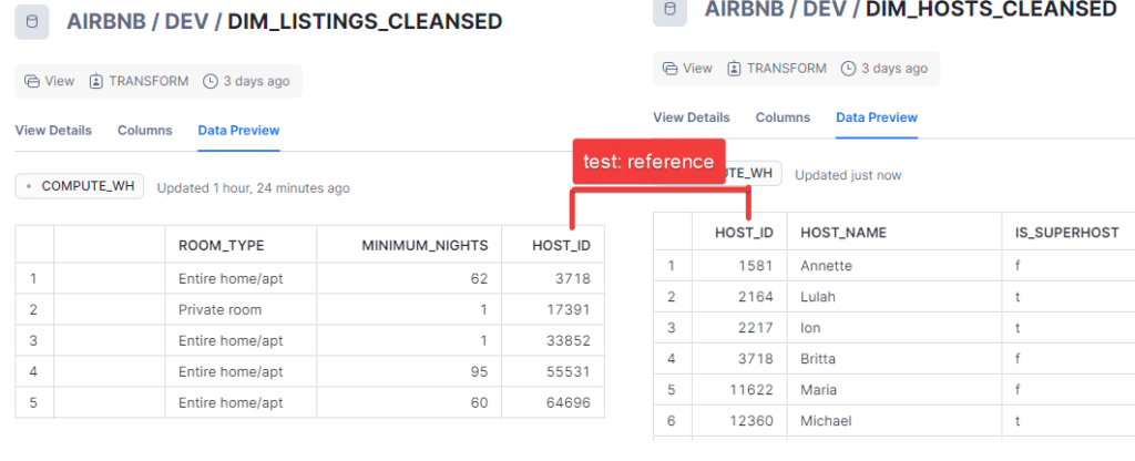
Built-in Test 4. relationships
In the relationships test, we will ensure that each id in HOST_ID in DEV.DIM_LISTING_CLEANSED has a reference in DEV.DIM_HOSTS_CLEANSED
To implement this test, we can use the following code in our scehma.yml file. Since we are creating a reference relationship to dim_hosts_cleansed based on field host_id in that table. The entry will be :
      - name: host_id
        test:
          -not_null
          -relationships:
            to: ref('dim_hosts_cleansed')
            field: host_id
Now when we run dbt test, we see the fourth test added.
Implementing Singular Tests
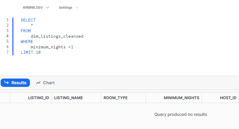
A singular test consists of an SQL query which passes when no rows are returns, or , the test fails if the query returns result. It is used to validate assumptions about data in a specificmodel. We implement singular tests by writing sql query in sql file in tests folder ,case dim_listings_minimum_night.sql
We will check in the test whether there are any minimum nights = 0 in the table. If there are none , result will return no rows and our test will pass.
Checking in snowflake itself , we get zero rows :
The test we have written in tests/dim_listings_minimum_nights.sql
-- tests/dim_listings_minimum_nights.sql
SELECT *
FROM {{ ref('dim_listings_cleansed') }}
WHERE minimum_nights <1
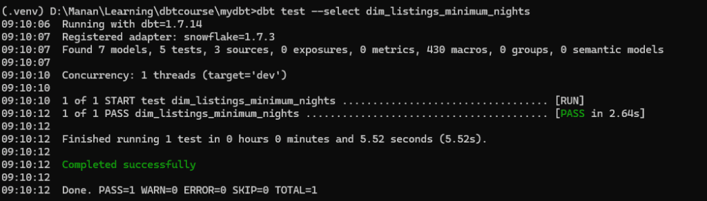
We can now implement the same test in dbt and run dbt test. In this case, I am executing a single test only. The output for which will become.
Since the resultset of the query was empty, therefore, the test passed. ( In other words, we were checking for exception, it did not occur, therefore test passed).
Implementing Custom Generic Tests
Custom Generic tests are tests which can accept parameters. They are defined in SQL file and are identified by parameter {% test %} at the beginning of the sql file. Lets write 2 tests using two different methods supported by DBT.
Custom Generic Test with Macros
First, we careate a .sql file under macros folder . In this case we are creating macros/positive_value.sql. The test accepts two parameters and then returns rows if the column name passed in parameters has value of less than 1.
{% test positive_value(model,column_name) %}

SELECT
*
FROM
    {{model}}
WHERE
    {{column_name}} < 1

{% endtest %}
After writing the test, we will specify the test within schema.yml file
To contrast the difference between Generic in-built test and Generic custom test, lets review the schema.yml configuration.
We have defined two tests on column minimum_nights. First was built-in not_null test that we did in last section. In this section, we created a macro by the name of positive_value(model,column_name) . The macro accepted two parameters. Both these parameters will be passed from schema.yml file . It will look up the model under which macro is specified and pass on that model. Similarly, it will pass on the column_name under which macro is mentioned.
Its important to remember that whether the test is defined in macros or is in-built. Test is passed only when no rows are returned. If any rows are returned, test will fail.
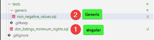
Custom Generic Test with generic subfolder
The other way of specifying custom generic test is under tests/generic. Also remember that we create a singular test under tests folder. Here’s a visual indication of the difference.
Singular tests are saved under tests/
Customer generic tests are saved under tests/generic
Since its a generic test, it will start with the {% test %} . The code for our test is
-- macros/tests/generic/non_negative_value.sql

{% test non_negative_value(model, column_name) %}
SELECT
  *
FROM
  {{ model }}
WHERE
  {{ column_name }} < 0
{% endtest %}
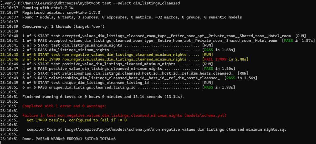
I want to implement this test on listing_id in dim_listings_cleansed. And I also want the test to fail. ( just to clarify the concept).I will go to schema.yml and define the test under column listing_id.
When I now run dbt test, DBT finds the test under macros/generic, however, it fails the test because there are several rows returned
Conclusion
In this hands-on exploration, we implemented various DBT testing methods to ensure data quality and reliability. We implemented built-in schema tests for core data properties, created reusable custom generic tests, and wrote singular tests for specific conditions. By leveraging these techniques, we can establish a robust testing strategy that safeguards our data warehouse, promotes high-quality data, and strengthens the foundation for reliable data pipelines.
In this article we will follow along complete dbt(Data Build Tool) bootcamp to create an end-to-end project pipeline using DBT and Snowflake. We begin by outlining the steps we will be performing in this hands-on project.
1.Loading Data from AWS to Snowflake:
Data from S3 is loaded into Snowflake using the COPY INTO command.
The raw data is stored in a dedicated schema (Airbnb.RAW).
2. Configuring Python & DBT:
Set up a virtual environment and install dbt-snowflake.
Create a user in Snowflake with appropriate permissions.
Initialize a dbt project and connect it to Snowflake.
3. Creating Staging Layer Models:
Models in dbt are SQL files representing transformations.
Staging models transform raw data into a cleaner, more structured format.
Use dbt commands to build and verify models.
4. Creating Core Layer Models & Materializations:
Core models apply further transformations and materializations.
Understand different materializations like views, tables, incremental, and ephemeral.
Create core models with appropriate materializations and verify them in Snowflake.
5. Creating DBT Tests:
Implement generic and custom tests to ensure data quality.
Use source freshness tests to monitor data timeliness.
6. Creating DBT Documentation:
Document models using schema.yml files and markdown files.
Generate and serve documentation to provide a clear understanding of data models and transformations.
The complete sources and code for this article can be found from the original course here.
Lets begin the hands-on implementation step by step.
We have now sourced the raw data that we want to build our data pipeline on.
2.Configuring Python & DBT
Next step is to create a temporary staging area to store the data without transformations . Since downstream processing of data can put considerable load on the systems, this staging area helps in decoupling the load. It also helps in auditing purposes.
In first step, we created 3 tables in RAW schema manually and copied data into them. In this step, we will use DBT to create staging area .
Setting up Python and Virtual Enviornment
The first step we need to do is to setup python and a virtual enviornment. You can use global enviornment as well. However, it is preferred to go with virtual enviornment. I am using Visual studio code for this tutorial and assuming that you can configure VS code with a Virtual enviornment, therefore, not going into its detail. If you need help setting it up, please follow this guide for setup.
After setting up virtual enviornment, please intall dbt-snowflake. DBT has adapters ( packages) for several data warehouses. Since we are using Snowflake in this example, we will use the following package :
pip install dbt-snowflake
Creating user in Snowflake
To connect to Snowflake, we created a user dbt in snowflake, granted it role called transform and granted “ALL” priveleges on database Airbnb. ( This is by no means a standard or recommended practice, we will do all blanket priveleges only for the purpose of this project). We use the following SQL in Snowflake to create a user and grant privileges.
-- Create the `dbt` user and assign to role
CREATE USER IF NOT EXISTS dbt
  PASSWORD='dbtPassword123'
  LOGIN_NAME='dbt'
  MUST_CHANGE_PASSWORD=FALSE
  DEFAULT_WAREHOUSE='COMPUTE_WH'
  DEFAULT_ROLE='transform'
  DEFAULT_NAMESPACE='AIRBNB.RAW'
  COMMENT='DBT user used for data transformation';
GRANT ROLE transform to USER dbt;


-- Set up permissions to role `transform`
GRANT ALL ON WAREHOUSE COMPUTE_WH TO ROLE transform;
GRANT ALL ON DATABASE AIRBNB to ROLE transform;
GRANT ALL ON ALL SCHEMAS IN DATABASE AIRBNB to ROLE transform;
GRANT ALL ON FUTURE SCHEMAS IN DATABASE AIRBNB to ROLE transform;
GRANT ALL ON ALL TABLES IN SCHEMA AIRBNB.RAW to ROLE transform;
GRANT ALL ON FUTURE TABLES IN SCHEMA AIRBNB.RAW to ROLE transform;
Now that we have the credentials for Snowflake, we can provide this information to dbt for connection.
Creating DBT Project
Once dbt-snowflake and its required dependencies are installed, you can now proceed with setting up dbt project. Inside the virtual enviornment , initiate the dbt core project with dbt init [project name]
dbt init mydbt
In my case , I am building this dbt project within DBTCOURSE folder, I will name my dbt core project as mydbt, therefore, my folder structure would be :
DBTCOURSE -> mydbt > ALL DBT FOLDERS AND FILES
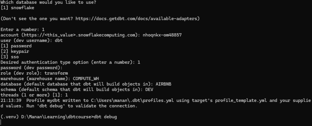
Since its the first time we are running dbt init, it will ask the name of the project, the database we are connecting to and the authentication credentials for the platform ( snowflake) .
Connecting DBT to Snowflake
After project is initiated, DBT will ask for user access credentials to connect to Snowflake with appropriate permissions on the database and schema’s we want to work on. Given below is summary of information command prompt will ask to connect.
Prompt
Value
platform ( number)
[1] Snowflake
account
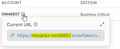
This is your Snowflake account identifier.
user
User we created to connect to snowflake ( dbt in this case)
password
user’s password
role
Role we assigned to the above user, that we want dbt to open the connection with
database
Database we want our connection established with (AIRBNB in this case )
schema
This is the default schema where dbt will build all models ( DEV in this case )
At times, finding Snowflake’s account identifier can be tricky. you can find it from Snowflake > Admin > Account > Hover over the account row.
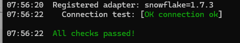
Verifying DBT connection
We can verify whether our dbt project has been configured properly and that it is able to connect to Snowflake using the dbt debug
dbt debug
The verbose output is quite long, however, I have provided screenshots only of key checks which enable us to start working with our project.
3.Creating data models in Staging Layer with DBT
Concept : Models in DBT
In dbt (Data Build Tool), models are SQL files that contain SELECT statements. These models define transformations on your raw data and are the core building blocks of dbt projects. Each model represents a transformation step that takes raw or intermediate data, applies some logic, and outputs the transformed data as a table or view in your data warehouse.Models promote modularity by breaking down complex transformations into simpler, reusable parts. This makes the transformation logic easier to manage and understand.
We will explore how models in dbt function within a dbt project to build and manage a data warehouse pipeline. An overview of key model characteristics and functions we will look at are :
Data Transformation: Models allow you to transform raw data into meaningful, structured formats. This includes cleaning, filtering, aggregating, and joining data from various sources.
Incremental Processing: Models can be configured to run incrementally, which means they only process new or updated data since the last run. This improves efficiency and performance.
Materializations:
Models in dbt can be materialized in different ways:
Views: Create virtual tables that are computed on the fly when queried.
Tables: Persist the transformed data as physical tables in the data warehouse.
Incremental Tables: Only update rows that have changed or been added since the last run.
Ephemeral: Used for subqueries that should not be materialized but instead embedded directly into downstream models.
Testing: dbt allows usto write tests for your models to ensure data quality and integrity. These can include uniqueness, non-null, and custom tests that check for specific conditions.
Documentation: Models can be documented within dbt, providing descriptions and context for each transformation. This helps in understanding the data lineage and makes the project more maintainable.
Dependencies and DAGs: Models can reference other models using the ref function, creating dependencies between them. dbt automatically builds a Directed Acyclic Graph (DAG) to manage these dependencies and determine the order of execution.
Version Control: Because dbt models are just SQL files, they can be version controlled using Git or any other version control system, enabling collaboration and change tracking.
Concept: Staging Layer
Staging layer is an abstraction used to denote purpose of data models in enterprise data warehouses. The concept of staging layer is prevalent in both Kimball and Inmon methodologies for data modeling . For dbt purposes, we will use a folder src under models to create the staging layer. Using staging layer we decouple the source data for further processing. In staging layer we create 3 simple models under models/src/
#
Model
Transformation
Materialization
1
Airbnb.DEV.src_listing
Column name changes
View
2
Airbnb.DEV.src_reviews
Column name changes
View
3
Airbnb.DEV.src_hosts
Column name changes
View
Models in staging layer
Creating staging layer models
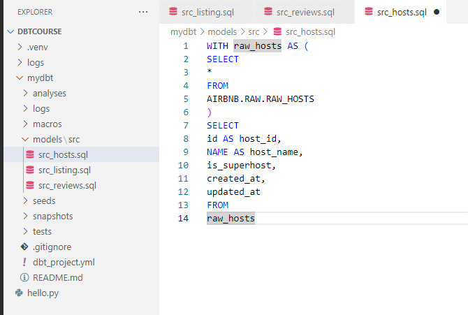
We create a new file src_listing.sql and use the following SQL to create our first model
WITH raw_listings AS (
SELECT
*
FROM
AIRBNB.RAW.RAW_LISTINGS
)
SELECT
id AS listing_id,
name AS listing_name,
listing_url,
room_type,
minimum_nights,
host_id,
price AS price_str,
created_at,
updated_at
FROM
raw_listings
We repeat the same for src_reviews and src_hosts
WITH raw_reviews AS (
SELECT
*
FROM
AIRBNB.RAW.RAW_REVIEWS
)
SELECT
listing_id,
date AS review_date,
reviewer_name,
comments AS review_text,
sentiment AS review_sentiment
FROM
raw_reviews
WITH raw_hosts AS (
SELECT
*
FROM
AIRBNB.RAW.RAW_HOSTS
)
SELECT
id AS host_id,
NAME AS host_name,
is_superhost,
created_at,
updated_at
FROM
raw_hosts
Our file structure after creating 3 models will be :
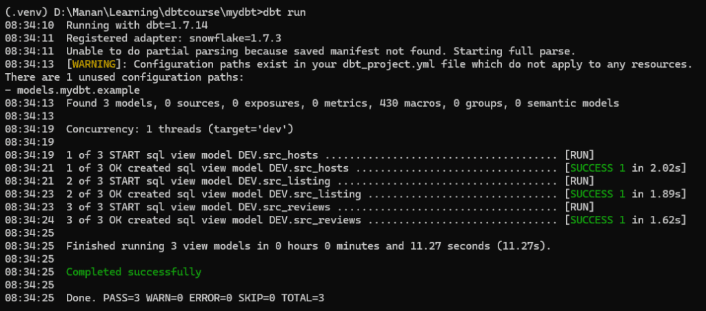
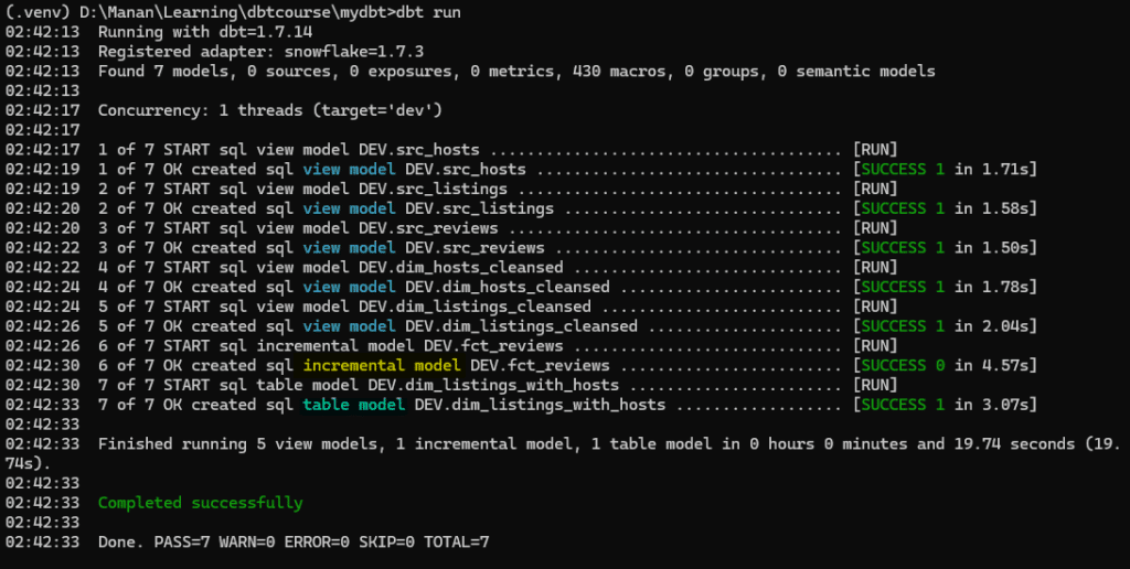
Finally, we can now run the dbt run command to build our first 3 models.
dbt run
It will start building models and in case there’s any error, it will show it. In case of succesful run, it will confirm on the prompt.
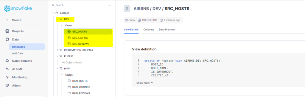
To confirm the models in our Snowflake database, we can now navigate to Snowflake and see whether our new models appear there .
As you can see , dbt has succesfully created 3 new models under AIRBNR.DEV schema, thus completing our staging layer.
4.Creating core layer models & materializations
In this step , we will create the “Core” layer with three models. We will also explore materializations in dbt and make a choice of which materializations we want our models to have. A summary of models we will create in this step alongside their materialization choice is :
Dbt supports four types of materialization. We can specify the materialization of a model either in the model file ( .sql) or within the dbt-project.yaml file. For our excercise, we will use both approaches to get familiar with both.
A comparative view of materializations supported by dbt and when to use them is as follows:
Feature
View
Table
Incremental
Ephemeral
Description
Creates a virtual table that is computed on the fly when queried.
Creates a physical table that stores the results of the transformation.
Updates only the new or changed rows since the last run.
Creates temporary subqueries embedded directly into downstream models.
Use Case
Use when you need to frequently refresh data without the need for storage.
Use when you need fast query performance and can afford to periodically refresh the data.
Use when dealing with large datasets and only a subset of the data changes frequently.
Use for intermediate transformations that don’t need to be materialized.
Pros
– No storage costs.<br>- Always shows the latest data.<br>- Quick to set up.
– Fast query performance.<br>- Data is stored and doesn’t need to be recomputed each time.
– Efficient processing by updating only changed data.<br>- Reduces processing time and costs.
– No storage costs.<br>- Simplifies complex transformations by breaking them into manageable parts.
Cons
– Slower query performance for large datasets.<br>- Depends on the underlying data’s performance.
– Higher storage costs.<br>- Requires periodic refreshing to keep data up-to-date.
– More complex setup.<br>- Requires careful handling of change detection logic.
– Can lead to complex and slow queries if overused.<br>- Not materialized, so each downstream query must recompute the subquery.
Materializations in dbt
Creating Core Layer models
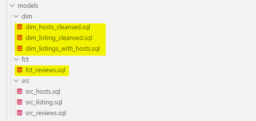
We will apply transformation to our staging layer models and create core layer models as discussed above. Our project structure after creating these models would change as shown below.
dim_hosts_cleansed
{{
config(
materialized = 'view'
)
}}
WITH src_hosts AS (
SELECT
*
FROM
{{ ref('src_hosts') }}
)
SELECT
host_id,
NVL(
host_name,
'Anonymous'
) AS host_name,
is_superhost,
created_at,
updated_at
FROM
src_hosts
dim_listing_cleansed
WITH src_listings AS (
SELECT
*
FROM
{{ ref('src_listings') }}
)
SELECT
listing_id,
listing_name,
room_type,
CASE
WHEN minimum_nights = 0 THEN 1
ELSE minimum_nights
END AS minimum_nights,
host_id,
REPLACE(
price_str,
'$'
) :: NUMBER(
10,
2
) AS price,
created_at,
updated_at
FROM
src_listings
dim_listings_with_hosts
WITH
l AS (
SELECT
*
FROM
{{ ref('dim_listings_cleansed') }}
),
h AS (
SELECT *
FROM {{ ref('dim_hosts_cleansed') }}
)
SELECT
l.listing_id,
l.listing_name,
l.room_type,
l.minimum_nights,
l.price,
l.host_id,
h.host_name,
h.is_superhost as host_is_superhost,
l.created_at,
GREATEST(l.updated_at, h.updated_at) as updated_at
FROM l
LEFT JOIN h ON (h.host_id = l.host_id)
fct_reviews
{{
config(
materialized = 'incremental',
on_schema_change='fail'
)
}}
WITH src_reviews AS (
SELECT * FROM {{ ref('src_reviews') }}
)
SELECT * FROM src_reviews
WHERE review_text is not null
{% if is_incremental() %}
AND review_date > (select max(review_date) from {{ this }})
{% endif %}
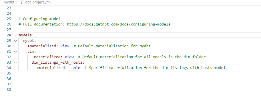
In our models above, we have explicitly created materialization configuration within the models for fct_reviews and dim_hosts_cleansed. For the others, we have used dbt-project.yaml file to specify the materialization.
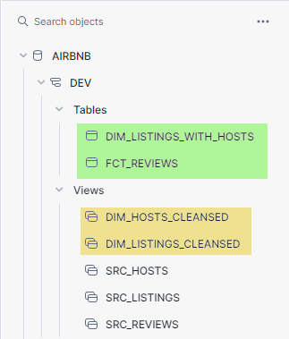
With the above materialization specifications within the Yaml file, we run the dbt and get the following output.
We can check the same in Snowflake interface , which will show us the new models created.
Adding sources to the models
Concept : Source in DBT
Sources in dbt are aliases given to the actual tables. Its an additional abstraction added over external tables which makes it possible to name and describe the data loaded into warehouse. Sources enable the following :
We can calculate the freshness of source data.
Test our assumptions about source data
select from source tables in our models using {{source()}} function , this helps in defining lineage of data.
Adding Sources
To add sources to our model, we will create a file “sources.yml” ( Filename is arbitrary ) . Once we have created config file , we can now go in to src_* files and replace existing table names with our “sources”.
A benefit of using “sources” in DBT is to be able to maintain freshness of data. Source freshness is a mechanism in DBT which enables monitoring the timeliness and update frequency of data in our sources. Source freshness mechanism allows for “warning” or “error” as notification mechanism for data freshness.
Here are the steps to configure source freshness.
In our sources.yml file, we decide a “date/time” field which acts as the cut-off point for source monitoring(loaded_at_field).
We specify a maximum allowable data age ( in interval e.g. hours or days) before a warning or error is triggered.(warn_after or warn_before)
We execute dbt source freshness command to check the freshness of sources.
If the data exceeds the freshness thresholds, DBT raises warnings or errors.
Here is what we have told the above yml file to do.
Parameter
Setting
Description
loaded_at_field
date
Check in “date” field when was data last loaded
warn_after
{count: 1, period: hour}
Issues a warning if the data in the date field is older than 1 hour.
error_after
{count: 24, period: hour}
Issues an error if the data in the date field is older than 24 hours.
source freshness configuration
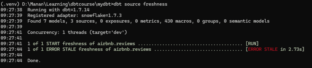
Now when we go to command prompt and run:
dbt source freshness
We get the following output
Creating tests in DBT
Concept: DBT tests
Dbt provides a comprehensive test framework to ensure data quality and reliability. Here’s a summary of tests that dbt supports.
Test Type
Subtype
Description
Usage
Implementation method
Generic Tests
Built-in
Pre-built or out-of-the-box tests for common data issues such as uniqueness, not-null, and referential integrity.
unique, not_null, relationships,accepted_values
schema.yml using tests: key under model/column
Custom Generic Tests
Custom tests written by users that can be applied to any column or model, similar to built-in tests but with custom logic.
Custom reusable tests with user-defined SQL logic.
1. Dbt automatically picks up from tests/generic/test_name.sql starting with {% tests %} . 2. Schema.yml by defining tests in .sql file and applying in schema.yml 3.macros: Historically, this wa the only place they could be defined.
Singular Tests
Designed to validate a single condition and are not intended to be reusable e.g. check if total sales reported in a period matches the sum of individual sales record.
Custom SQL conditions specific to a model or field.
Dbt automatically picks up test from tests/test_name.sql
Source Freshness Tests
Tests that check the timeliness of the data in your sources by comparing the current timestamp with the last updated timestamp.
dbt source freshness to monitor data update intervals.
Schema.yml using freshness: key under source/table
DBT testing framework
Implementing Built-In Tests
We will begin by writing generic tests. To improve the readability of this article, I have moved the testing to an article of its own, please continue with implementing Built-In tests on this link.
Documenting models in DBT
In any data warehousing project, documentation act as a blueprint and reference guide for data structures. It should capture key information about data models essentially explaining what data is stored, how it is organised and how does it relate to other data. DBT solves the problem of documenting models by providing framework for implementing documentation within its own framework.
Writing documentations for our Models
DBT provides two methods for writing documentation. We can either write the documentation within the schema.yml file as text or we can write documentation in separate markup files and link them back to schema.yml file. We will explore both these options. Please follow this link to see hands-on documentation in DBT.
Conclusion
In this article, we created an end-to-end project pipeline using dbt and Snowflake. DBT makes it easier for data engineers to effectively build and manage reliable and scalable data pipelines. We started by loading data from S3 into Snowflake using the COPY INTO command, storing the raw data in a dedicated schema (Airbnb.RAW). Next, we configured Python and dbt, setting up a virtual environment, installing dbt-snowflake, creating a user in Snowflake with appropriate permissions, and initializing a dbt project connected to Snowflake. We then created staging layer models, which are SQL files representing transformations, to clean and structure the raw data. Using dbt commands, we built and verified these models. Moving on to the core layer, we applied further transformations and materializations, exploring different types like views, tables, incremental, and ephemeral. We created core models with appropriate materializations and verified them in Snowflake. To ensure data quality, we implemented generic and custom tests, as well as source freshness tests to monitor data timeliness. Lastly, we documented our models using schema.yml files and markdown files, generating and serving the documentation to provide a clear understanding of data models and transformations. By following these steps, data engineers can leverage dbt to build scalable and maintainable data pipelines, ensuring data integrity and ease of use for downstream analytics.
Slowly Changing Dimensions (SCDs) are an approach in data warehousing used to manage and track changes to dimensions over time. It plays an important role in data modeling especially in the context of a data warehouse where maintaining historical accuracy of data over time is essential. The term “slow” in SCDs refer to rate of change and the method of handling these changes. For example, changes to a customer’s address or marital status happen infrequently, making these “slowly” changing dimensions. This is in contrast to “fast-changing” scenarios where data elements like stock prices or inventory levels might update several times a day or even minute by minute.
Types of SCDs
In the context of data modeling, there are 3 types of slowly changing dimensions. Choosing the right type of SCD depends on business requirements. Given below is brief overview of the most frequently used types of SCDs in data modeling
Type 1 SCD (No History)
Overwrites old data with new data. It’s used when the history of changes isn’t necessary. For example, correcting a misspelled last name of a customer.
In this table Manan’s email address is updated directly in the database, replacing the old email with the new one. No historical record of old mail is maintained.
Type 2 SCD (Full History)
Adds new records for changes, keeping historical versions. It’s crucial for auditing purposes and when analyzing the historical context of data, like tracking price changes over time.
Scenario:
A customer changes their subscription plan.
Before the Change:
Originally, the customer is subscribed to the “Basic” plan.
Customer ID
Name
Subscription Plan
Start Date
End Date
Current
001
Manan Younas
Basic
2023-01-01
NULL
Yes
After the Change:
The customer upgrades to the “Premium” plan on 2023-06-01.
Update the existing record to set the end date and change the “Current” flag to “No.”
Add a new record with the new subscription plan, starting on the date of the change.
Customer ID
Name
Subscription Plan
Start Date
End Date
Current
001
John Doe
Basic
2023-01-01
2023-06-01
No
001
John Doe
Premium
2023-06-01
NULL
Yes
Explanation:
Before the Change: The table shows John Doe with a “Basic” plan, starting from January 1, 2022. The “End Date” is NULL, indicating that this record is currently active.
After the Change: Two changes are made to manage the subscription upgrade:
The original “Basic” plan record is updated with an “End Date” of January 1, 2023, and the “Current” status is set to “No,” marking it as historical.
A new record for the “Premium” plan is added with a “Start Date” of January 1, 2023. This record is marked as “Current” with a NULL “End Date,” indicating it is the active record.
This method of handling SCDs is beneficial for businesses that need to track changes over time for compliance, reporting, or analytical purposes, providing a clear and traceable history of changes.
Type 3 SCD (Limited History)
Type 3 SCDs add new columns to store both the current and at least one previous value of the attribute, which is useful for tracking limited history without the need for multiple records.It is less commonly used but useful for tracking a limited history where only the most recent change is relevant.
Scenario:
A customer moves from one city to another.
Before the Move:
Initially, only current information is tracked.
Customer ID
Name
Current City
001
Manan Younas
Sydney
After the Move:
A new column is added to keep the previous city alongside the current city.
Customer ID
Name
Current City
Previous City
001
Manan Younas
Melbourne
Sydney
Explanation:
In this table, when Manan moves from Sydney to Melbourne, the “Current City” column is updated with the new city, and “Previous City” is added to record his last known location. This allows for tracking the most recent change without creating a new record.
These examples illustrate the methods by which Type 1 , Type2 and Type 3 SCDs manage data changes. Type 1 SCDs are simpler and focus on the most current data, discarding historical changes. Type 3 SCDs, meanwhile, provide a way to view a snapshot of both current and previous data states without maintaining full historical records as Type 2 SCDs do.
Architectural considerations for Managing SCDs
The management of Slowly Changing Dimensions (SCDs) in data warehousing requires careful architectural planning to ensure data accuracy, completeness, and relevance. Lets discuss the implementation considerations for each type of SCD and the architectural setups required to support these patterns effectively.
Type 1 Implementation consideration
Scenarios Where Most Effective
Type 1 SCDs are most effective in scenarios where historical data is not needed for analysis and only the current state is relevant. Common use cases include:
Correcting data errors in attributes, such as fixing misspelled names or incorrect product attributes.
Situations where business does not require tracking of historical changes, such as current status updates or latest measurements.
Architectural Setup
Database Design: A simple design where each record holds the latest state of the data. Historical data tracking mechanisms are not needed.
Data Update Mechanism: The implementation requires a straightforward update mechanism where old values are directly overwritten by new ones without the need for additional fields or complex queries.
Performance Considerations: Since this pattern only involves updating existing records, it typically has minimal impact on performance and does not significantly increase storage requirements.
Type 2 Implementation consideration
Scenarios Where Most Effective
Type 2 SCDs are crucial when the full history of changes must be preserved for compliance, reporting, or analytical purposes. They are widely used in:
Customer information management, where it is necessary to track address history, status changes, or subscription details.
Product information tracking, where changes over time can provide insights into lifecycle management and evolution.
Architectural Setup
Database Design: Requires a more complex setup with additional fields for managing historical data, such as start date, end date, and a current flag.
Data Management Strategy: Insertion of new records for each change, while updating or closing previous records to indicate they are no longer current. This setup can be managed through triggers or application logic.
Versioning and Timestamping: Implementation of version control and timestamping to ensure each change is accurately recorded with its validity period.
Performance and Storage Considerations: Type 2 can significantly increase the volume of data stored, which may impact performance. Indexing on key fields and partitioning historical data can help optimize query performance.
Type 3 Implementation Pattern
Scenarios Where Most Effective:
Type 3 SCDs are used when tracking a limited history is sufficient. This can be applicable in cases like:
Tracking a previous address alongside the current one for a short-term promotional campaign.
Monitoring recent changes in terms and conditions for services, where only the most recent previous state is relevant.
Architectural Setup:
Database Design: Includes additional columns to store both the current and previous values of the tracked attributes. This setup is simpler than Type 2 but more complex than Type 1.
Data Update Mechanism: Updates involve changing multiple fields within a single record—both updating the previous value fields and writing new current values.
Performance Considerations: This method increases the size of each record but does not increase the total number of records as Type 2 does. Performance impacts are generally moderate but can involve more complex queries than Type 1.
Conclusion
Each type of SCD requires a different architectural approach based on the business requirements for historical data. While Type 1 is simpler and less resource-intensive, Types 2 and 3 provide data tracking capabilities at the cost of additional complexity and potentially higher resource requirements. Properly choosing and implementing these patterns will depend on the specific needs of the business, the criticality of historical data, and the performance impacts on the data warehouse system.
Association Rule Learning is used to find relationships between items or events in large data sets. The primary goal of Association Rule Learning is to identify frequently occurring patterns in data to reveal hidden relationships.
How Association Rule Learning works?
Association rules are typically represented in the form of “If {A} then {B}”, where A and B are sets of items or events. The strength of an association rule is usually measured by three key metrics:
Support: The proportion of transactions in the dataset that contain both A and B. A high support value indicates that the rule occurs frequently in the data.
Confidence: The probability of B occurring given that A has occurred. A high confidence value means that if A is present, there is a high likelihood of B also being present.
Lift The ratio of the observed support to the expected support if A and B were independent events. A lift value greater than 1 indicates that the occurrence of A and B together is more frequent than what would be expected if they were unrelated.
Use cases in Marketing Analytics
There are several applications of the Association Learning Rule, in the context of marketing analytics, listed below is a list of common use cases, their examples, and a very brief summary of how Association Rules are used in them.
wdt_ID
Category
Use Case
Example
Association Rule
1
Cross-channel Marketing
Channel strategy optimization
Identifying effective combinations of marketing channels for engagement or conversions
If {Email, Social_Media, Paid_Search} then {High_Conversions}
2
Email Marketing
Content and offer optimization
Identifying effective content and discount code combinations
If {Product_A_Recommendation} then {Discount_Code_X}
3
Content Marketing
Content strategy optimization
Identifying popular combinations of blog topics to engage users
If {Blog_Topic_A, Blog_Topic_B} then {High_Engagement}
4
Social Media Marketing
Social media strategy optimization
Finding effective combinations of social media posts, hashtags, or influencers
If {Post_Type_A, Hashtag_X} then {High_Engagement}
5
Search Engine Optimization (SEO)
SEO strategy optimization
Identifying effective combinations of keywords and content types for organic traffic
If {Keyword_A, Content_Type_B} then {High_Organic_Traffic}
6
Landing Page Optimization
Conversion optimization
Analyzing the effectiveness of different landing page elements
If {Image_A, Headline_B, CTA_C} then {High_Conversions}
7
Affiliate Marketing
Affiliate strategy optimization
Identifying the most effective combinations of affiliate offers and traffic sources
If {Affiliate_Offer_A, Traffic_Source_B} then {High_Conversions}
8
Online Advertising
Ad strategy optimization
Analyzing the impact of different ad creatives and targeting options
If {Ad_Creative_A, Targeting_B} then {High_Clicks}
9
Customer Segmentation
Targeted marketing optimization
Analyzing associations between customer attributes and marketing responsiveness
If {Demographics_A, Browsing_Behavior_B} then {High_Engagement}
10
Product Recommendations
Personalization
Analyzing associations between products in an online store to inform recommendations
If {Product_A, Product_B} then {High_Likelihood_of_Purchase}
Algorithms for Association Rule Learning
To get an idea of various algorithms based on Association Rule Learning, given below is a summary of such algorithms developed over the last 3 decades.
Association Rule Learning – Algorithms Summary
Algorithm
wdt_ID
What it does
Developed by
Year of development
Total Citations
Apriori
1
Mines frequent itemsets using a breadth-first search
Rakesh Agrawal, Tomasz Imieliński, Arun Swami
1993
~22,000
Eclat
2
Mines frequent itemsets using a depth-first search
Mohammed J. Zaki
1997
~3,000
FP-Growth
3
Mines frequent itemsets without candidate generation
Jiawei Han, Jian Pei, Yiwen Yin
2000
~12,000
H-mine
4
Improves upon FP-growth using a hyper-structure approach
J. Pei, J. Han, H. Lu, S. Nishio, S. Tang, D. Yang
2001
~800
RElim
5
Eliminates items recursively to mine frequent itemsets
Christian Borgelt
2004
~200
LCM
6
Mines closed frequent itemsets in linear time
Takeaki Uno, Tatsuya Asai, Hiroki Arimura
2004
~400
FARMER
7
Uses a matrix-based data structure to mine frequent itemsets
Roberto J. Bayardo Jr.
2004
~100
OPUS Miner
8
Discovers the top-K association rules with the highest overall utility
Vertex AI is Google’s solution for problem-solving in Artificial Intelligence domain. To put things into context, Microsoft provides Azure Machine Learning platform for artificial intelligence problem solving and Amazon has Sage Maker for solving AI workloads.
Google’s Vertex AI supports two processes for model training.
AutoML: This is the easy version. It lets you, train models with low effort and machine learning expertise. The downside is that the parameters you can tweak in this process are very limited.
Custom training: This is free space for data science engineers to go wild with machine learning. You can train models using TensorFlow, sickit-learn, XGBoost etc.
In this blog post, we will use AutoML to train a classification model, deploy it to a GCP endpoint, and then consume it using the GS cloud shell.
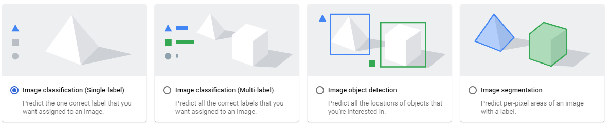
Supported data types
Image
Image classification single-label
Image classification multi-label
Image object detection
Image segmentation
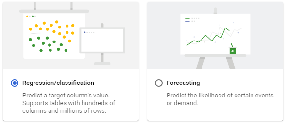
Tabular
Regression / classification
Forecasting
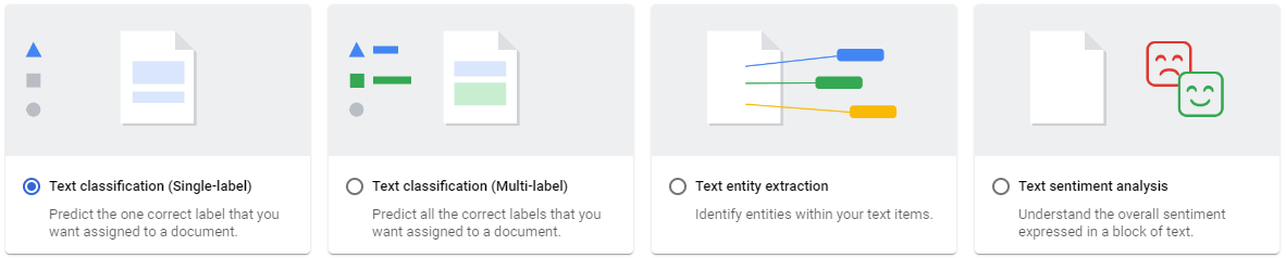
Text
Text classification single-label
Text classification Multi-label
Text entity extraction
Text sentiment analysis
Video
Video action recognition
video classification
video object tracking
Supported Data sources
You can upload data to Vertex AI from 3 sources
from Local computer
From google cloud storage
From Bigquery
Training a model using AutoML
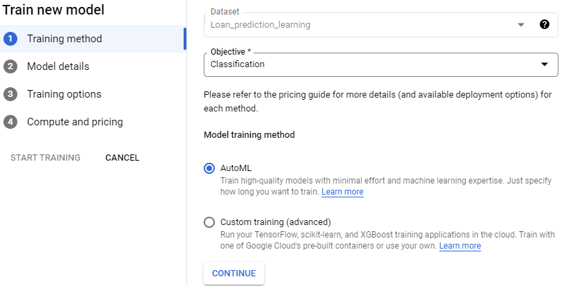
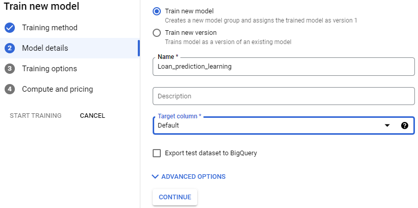
Training a model in AutoML is straightforward. Once you have created your dataset, you can use a click-point interface for creating a model.
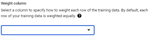
Training Method
Model Details
Training options
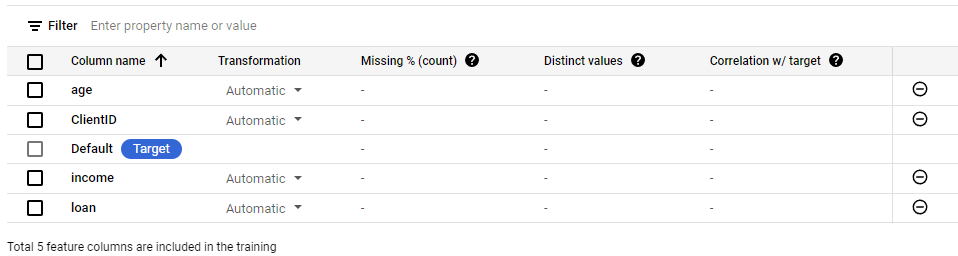
Feature Selection
Factor weightage
You have an option to weigh your factors equally.
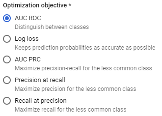
Optimization objective
Optimization objectives options vary for each workload type. In our case, we are doing classification, hence it has given options relevant to an optimization workload. For more details on optimzation objectives, this optimization objective documentation is very helpful.
Compute and pricing
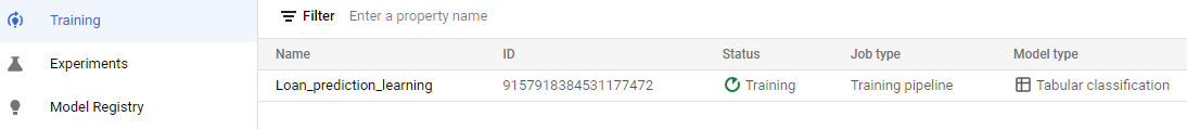
Lastly, we have to select Budget in terms of how many node hours do we want our model to run for. Google’s vertex AI pricing guide is helpful in understanding the pricing.
Once you have completed these steps, your model will move into training mode. You can view the progress from the Training link in the navigation menu. Once the training is finished, the model will start to appear in Model Registry.
Deploying the model
Model deployment is done via Deploy and Test tab on the model page itself.
Click on Deploy to End-point
Select a machine type for deployment
Click deploy.
Consuming the model
To consume the model, we need a few parameters. We can set these parameters as environment variables using the Google cloud shell and then invoke the model with ./smlproxy