MapReduce is a fundamental algorithmic model used in distributed computing to process and generate large datasets efficiently. It was popularized by Google and later adopted by the open-source community through Hadoop. The model simplifies parallel processing by dividing work into map and reduce tasks, making it easier to scale across a cluster of machines. Whether you’re working in big data or learning Apache Spark, understanding MapReduce helps in building a strong foundation for distributed data processing.
What Is MapReduce?
MapReduce is all about breaking a massive job into smaller tasks so they can run in parallel.
Map: Each worker reads a bit of the data and tags it with a key.
Reduce: Another worker collects all the items with the same tag and processes them.
That’s it. Simple structure, massive scale.
Why Was MapReduce Needed?
MapReduce emerged when traditional data processing systems couldn’t handle the explosive growth of data in the early 2000s, requiring a new paradigm that could scale horizontally across thousands of commodity machines. Given below is a brief rundown of what problems existed for handling Big Data and how MapReduce solved it.
Problem
MapReduce Solution
Data Volume Explosion: Single machines couldn’t handle terabytes/petabytes of data
Automatic data splitting and distributed processing across multiple machines
Network failures and system crashes
Built-in fault tolerance with automatic retry mechanisms and task redistribution
Complex load balancing requirements
Automated task distribution and workload management across nodes
Data consistency issues in distributed systems
Structured programming model ensuring consistent data processing across nodes
Manual recovery processes after failures
Automatic failure detection and recovery without manual intervention
Difficult parallel programming requirements
Simple programming model with just Map and Reduce functions
Poor code reusability in distributed systems
Standardized framework allowing easy code reuse across applications
Complex testing of distributed applications
Simplified testing due to the standardized programming model
Expensive vertical scaling (adding more CPU/RAM)
Cost-effective horizontal scaling by adding more commodity machines
Data transfer bottlenecks
Data locality optimization by moving computation to data
Schema-on-Read:
Schema-on-read is backbone of MapReduce. It means you don’t need to structure your data before storing it. Think of it like this:
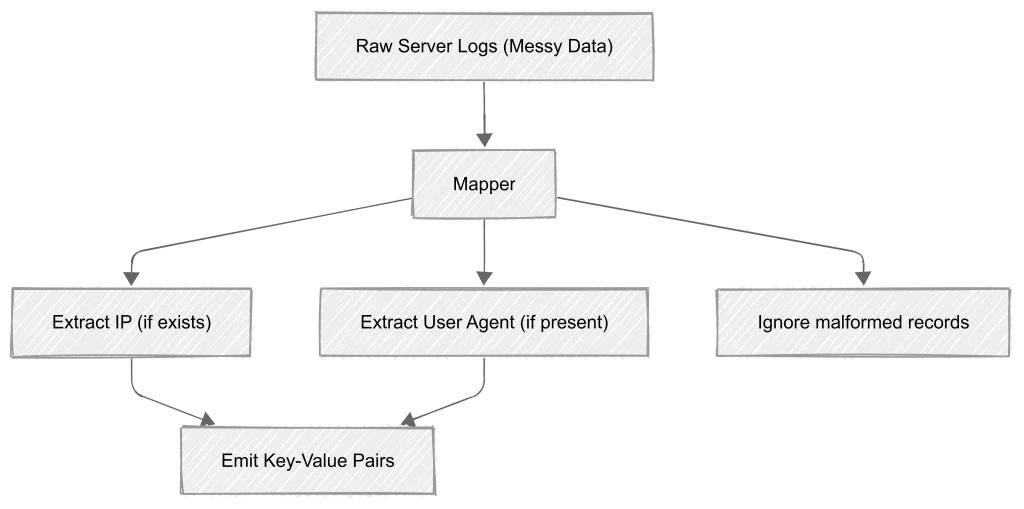
Your input data can be messy – log files, CSVs, or JSON – MapReduce doesn’t care
Mappers read and interpret the data on the fly, pulling out just the pieces they need
If some records are broken or formatted differently, the mapper can skip them and keep going
Example: Let’s say you’re processing server logs. Some might have IP addresses, others might not. Some might include user agents, others might be missing them. With schema-on-read, your mapper just grabs what it can find and moves on – no need to clean everything up first.
MapReduce doesn’t care what your data looks like until it reads it. That’s schema-on-read. Store raw files however you want, and worry about structure only when you process them.
How MapReduce Works in Hadoop
Let’s walk through a realistic example. Imagine a CSV file with employee info and we want to count the number of employees in each department :
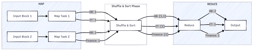
First, Hadoop splits the input file into blocks—say, 128MB each. Why? So they can be processed in parallel across multiple machines. That’s how Hadoop scales.
Each Map Task reads lines from its assigned block. In our case, each line represents an employee record, like this:
101, Alice, HR
What do we extract from this? It depends on our goal. Since we’re counting people per department, we group by department. That’s why we emit:
("HR", 1)
We don’t emit ("Alice", 1) because we’re counting departments, not individuals. This key-value pair structure prepares us perfectly for the reduce phase.
Step 2: Shuffle and Sort
These key-value pairs then move into the shuffle phase, where they’re grouped by key:
("HR", [1, 1])

("IT", [1])

("Finance", [1])
Step 3: Reduce
Each reducer receives one of these groups and sums the values:
("HR", 2)

("IT", 1)

("Finance", 1)
The final output shows the headcount per department.
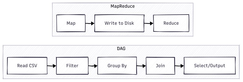
MapReduce Today: The Evolution to DAG-Based Processing
While MapReduce revolutionized distributed computing, its rigid two-stage model had limitations. Each operation required writing to disk between stages, creating performance bottlenecks. Apache Spark introduce the concept of DAG ( Directed Acyclic Graph)
The DAG model represents a fundamental shift in how distributed computations are planned and executed:
Flexible Pipeline Design: Instead of forcing everything into map and reduce steps, Spark creates a graph of operations that can have any number of stages
Memory-First Architecture: Data stays in memory between operations whenever possible, dramatically reducing I/O overhead
Intelligent Optimization: The DAG scheduler can analyze the entire computation graph and optimize it before execution
Lazy Evaluation: Operations are planned but not executed until necessary, allowing for better optimization
This evolution meant that while MapReduce jobs had to be explicitly structured as a sequence of separate map and reduce operations, Spark could automatically determine the most efficient way to execute a series of transformations. This made programs both easier to write and significantly faster to execute.
MapReduce vs. DAG: Comparison
Here’s a high level overview of how DAG in spark differs from MapReduce
Feature
MapReduce
DAG (Spark)
Processing Stages
Fixed two stages (Map and Reduce)
Multiple flexible stages based on operation needs
Execution Flow
Linear flow with mandatory disk writes between stages
Optimized flow with in-memory operations between stages
Job Complexity
Multiple jobs needed for complex operations
Single job can handle complex multi-stage operations
Performance
Slower due to disk I/O between stages
Faster due to in-memory processing and stage optimization
Key Advantages of DAG over MapReduce:
DAGs can optimize the execution plan by combining and reordering operations
Simple operations can complete in a single stage instead of requiring both map and reduce
Complex operations don’t need to be broken into separate MapReduce jobs
In-memory data sharing between stages improves performance significantly
This evolution from MapReduce to DAG-based processing represents a significant advancement in distributed computing, enabling more efficient and flexible data processing pipelines. For example you could use a much complex chaining of operations using a single line of code in multi-stage Dag as given below:
// Example of a complex operation in Spark creating a multi-stage DAG
val result = data.filter(...)
               .groupBy(...)
               .aggregate(...)
               .join(otherData)
               .select(...)
Understanding the Employee count Code Example
The employee count by department example we discussed above can be written in spark by using these 2 lines.
val df = spark.read.option("header", "true").csv("people.csv")
df.groupBy("department").count().show()
This code performs a simple but common data analysis task: counting employees in each department from a CSV file. Here’s what each part does:
Line 1: Reads a CSV file containing employee data, telling Spark that the file has headers
Line 2: Groups the data by department and counts how many employees are in each group
Let’s break down this Spark code to understand how it implements MapReduce concepts and leverages DAG advantages:
1. Schema-on-Read :
The line spark.read.option("header", "true").csv("people.csv") demonstrates schema-on-read – Spark only interprets the CSV structure when reading, not before.
It automatically detects column types and handles messy data without requiring pre-defined schemas.
2. Hidden Map Phase with DAG Optimization:
When groupBy("department") runs, Spark creates an optimized DAG of tasks instead of a rigid map-reduce pattern.
Each partition is processed efficiently with the ability to combine operations in a single stage when possible.
3. Improved Shuffle and Sort:
The groupBy operation triggers a shuffle, but unlike MapReduce, data stays in memory between stages.
DAG enables Spark to optimize the shuffle pattern and minimize data movement across the cluster.
4. Enhanced Reduce Phase:
The count() operation is executed as part of the DAG, potentially combining with other operations.
Unlike MapReduce’s mandatory disk writes between stages, Spark keeps intermediate results in memory.
5. DAG Benefits in Action:
The entire operation is treated as a single job with multiple stages, not separate MapReduce jobs.
Spark’s DAG optimizer can reorder and combine operations for better performance.
While the code looks simpler, its more than syntax simplification – the DAG-based execution model provides fundamental performance improvements over traditional MapReduce while maintaining the same logical pattern.
Code Comparison: Spark vs Hadoop MapReduce
Let’s compare how the same department counting task would be implemented in both Spark and traditional Hadoop MapReduce:
1. Reading Data
Spark:
val df = spark.read.option("header", "true").csv("people.csv")
Hadoop MapReduce:
public class EmployeeMapper extends Mapper<LongWritable, Text, Text, IntWritable> {
    private final static IntWritable one = new IntWritable(1);
    private Text department = new Text();

    public void map(LongWritable key, Text value, Context context) throws IOException, InterruptedException {
        String[] fields = value.toString().split(",");
        department.set(fields[2].trim());  // department is third column
        context.write(department, one);
    }
}
2. Processing/Grouping
Spark:
df.groupBy("department").count()
Hadoop MapReduce:
public class DepartmentReducer extends Reducer<Text, IntWritable, Text, IntWritable> {
    public void reduce(Text key, Iterable<IntWritable> values, Context context) throws IOException, InterruptedException {
        int sum = 0;
        for (IntWritable val : values) {
            sum += val.get();
        }
        context.write(key, new IntWritable(sum));
    }
}
3. Job Configuration and Execution
Spark:
// Just execute the transformation
df.groupBy("department").count().show()
Hadoop MapReduce:
public class DepartmentCount {
    public static void main(String[] args) throws Exception {
        Job job = Job.getInstance(new Configuration(), "department count");
        job.setJarByClass(DepartmentCount.class);

        job.setMapperClass(EmployeeMapper.class);
        job.setReducerClass(DepartmentReducer.class);

        job.setOutputKeyClass(Text.class);
        job.setOutputValueClass(IntWritable.class);

        FileInputFormat.addInputPath(job, new Path(args[0]));
        FileOutputFormat.setOutputPath(job, new Path(args[1]));

        System.exit(job.waitForCompletion(true) ? 0 : 1);
    }
}
Key Differences:
Spark requires significantly less boilerplate code
Hadoop MapReduce needs explicit type declarations and separate Mapper/Reducer classes
Spark handles data types and conversions automatically
Hadoop MapReduce requires manual serialization/deserialization of data types
Spark’s fluent API makes the data processing pipeline more readable and maintainable
Performance Implications:
Spark keeps intermediate results in memory between operations
Hadoop MapReduce writes to disk between map and reduce phases
Spark’s DAG optimizer can combine operations for better efficiency
Hadoop MapReduce follows a strict two-stage execution model
A vector in the context of NLP is a multi-dimensional array of numbers that represents linguistic units such as words, characters, sentences, or documents.
Motivation for Vectorisation
Machine learning algorithms require numerical inputs rather than raw text. Therefore, we first convert text into a numerical representation.
Tokens
The most primitive representation of language in NLP is a token. Tokenisation breaks raw text into atomic units – typically words, subwords or characters. These tokens form the basis of all downstream processing. A token is typically assigned a Token ID e.g. “Cat”—> 310 . However, tokens themselves carry no meaning unless they’re transformed into numeric vector.
Vectors
Although tokens and token IDs are numeric representations, they lack inherent meaning. To make these numbers meaningful mathematically, they are used as building blocks for vectors.
Vector is a mathematical representation in high-dimensional space. What that means is it carries more context than a bare number itself . As a simplified example , consider “cat”represented in a 5 dimension vector.
"cat" → [0.62, -0.35, 0.12, 0.88, -0.22]
Dimension
Value
Implied Meaning (not labeled in real models, just illustrative)
1
0.62
Animal-relatedness
2
-0.35
Wild vs Domestic (negative = domestic)
3
0.12
Size (positive = small)
4
0.88
Closeness to human-associated terms (like "pet", "owner", "feed")
5
-0.22
Abstract vs Concrete (negative = more physical/visible)
Embeddings
If we consider the our example of word "cat", its embedding vector consists of values that are shaped by exposure to language data—such as frequent co-occurrence with words like "meow", "pet", and "kitten". This contextual usage informs how the embedding is constructed, positioning "cat" closer to semantically similar words in the vector space.
More broadly, while vectors provide a numeric way to represent tokens, embeddings are a specialised form of vector that is learned from data to capture linguistic meaning. Unlike sparse or manually defined vectors, embeddings are dense, low-dimensional, and trainable.
Dimension
Value (Generic Vector)
Value (Embedding)
Implied Meaning (illustrative only)
1
0.62
0.10
Animal-relatedness
2
-0.35
0.05
Wild vs Domestic
3
0.12
-0.12
Size
4
0.88
0.02
Closeness to human-associated terms (e.g., pet, owner)
5
-0.22
-0.05
Abstract vs Concrete
Learned Embedding vs Generic Vector for "cat"
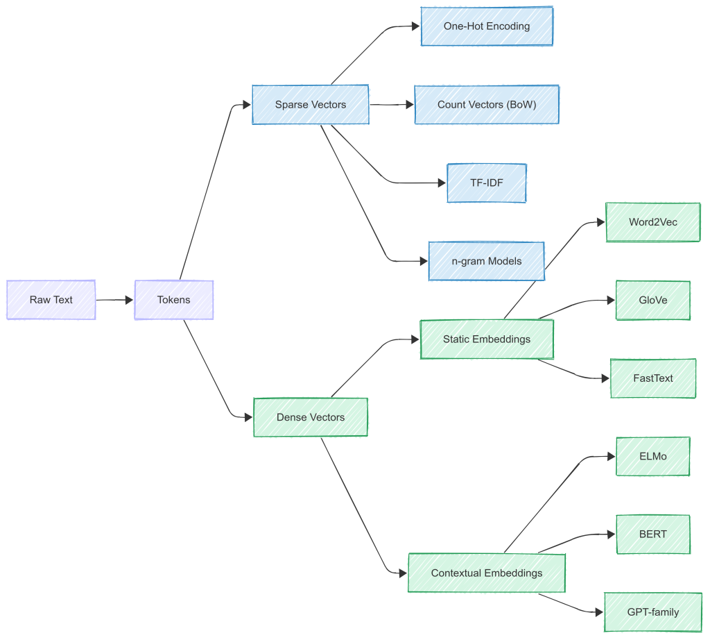
Vectorisation Algorithms
Given below is a brief summary of major vectorisation algorithms and their timeline.
Early Algorithms: Sparse Representations
Traditional NLP approaches like Bag of Words (BoW) and TF-IDF relied on token-level frequency information. They represent each document as a high-dimensional vector based on token counts.
Bag of Words (BoW)
Represents a document by counting how often each token appears.
Treats all tokens independently; ignores order and meaning.
Extends BoW by scaling down tokens that appear in many documents.
Aims to highlight unique or important tokens.
Output: still sparse and high-dimensional.
These approaches produce sparse vectors. As vocabulary size grows, vectors become inefficient and incapable of generalising across related words like "cat" and "feline."
Transition to Dense Vectors: Embeddings
To overcome the limitations of sparse representations, researchers introduced dense embeddings. These are fixed-size, real-valued vectors that place semantically similar words closer together in the vector space. Unlike count-based vectors, embeddings are learned through training on large corpora.
Early Embedding Algorithms – Dense Representation
Word2Vec (2013, Google – Mikolov)
Learns dense embeddings using a shallow neural network.
Words that appear in similar contexts get similar embeddings.
Two training strategies:
CBOW (Continuous Bag of Words): Predicts the target word from its surrounding context.
Skip-Gram: Predicts surrounding words from the target word.
Efficient training using negative sampling.
Limitation: Produces static embeddings. A word has one vector regardless of its context.
GloVe (2014, Stanford)
Stands for Global Vectors.
Learns embeddings by factorising a global co-occurrence matrix.
Combines global corpus statistics with local context windows.
Strength: Captures broader semantic patterns than Word2Vec.
Limitation: Still produces static embeddings.
Embedding Algorithms – Contextual Embeddings
Even though Word2Vec and GloVe marked a huge advancement, they had a major drawback: they generate one embedding per token, regardless of context. For example, the word "bank" will have the same vector whether it refers to a financial institution or a riverbank.
This limitation led to contextual embeddings such as:
ELMo (Embeddings from Language Models): Learns context from both directions using RNNs.
BERT (Bidirectional Encoder Representations from Transformers): Uses transformers to generate context-aware embeddings where each token’s representation changes depending on its surrounding words.
Spark provides three abstractions for handling data
RDDs
Distributed collections of objects that can be cached in memory across cluster nodes (e.g., if an array is large, it can be distributed across multiple clusters).
DataFrame
DataFrames are distributed collections of data organized into named columns, similar to tables in a relational database. They provide a powerful abstraction that supports structured and semi-structured data with optimized execution through the Catalyst optimizer.
DataFrames are schema-aware and can be created from various data sources including structured files (CSV, JSON), Hive tables, or external databases, offering SQL-like operations for data manipulation and analysis.
Dataset
Datasets are a type-safe, object-oriented programming interface that provides the benefits of RDDs (static typing and lambda functions) while also leveraging Spark SQL's optimized execution engine.
They offer a unique combination of type safety and ease of use, making them particularly useful for applications where type safety is important and the data fits into well-defined schemas using case classes in Scala or Java beans.
Comparison of Spark Data Abstractions
Feature
RDD
DataFrame
Dataset
Type Safety
Type-safe
Not type-safe
Type-safe
Schema
No schema
Schema-based
Schema-based
API Style
Functional API
Domain-specific language (DSL)
Both functional and DSL
Optimization
Basic
Catalyst Optimizer
Catalyst Optimizer
Memory Usage
High
Efficient
Moderate
Serialization
Java Serialization
Custom encoders
Custom encoders
Language Support
All Spark languages
All Spark languages
Scala and Java only
graph LR
    A["Data Storage in Spark"]

    A --> B["RDD"]
    A --> C["DataFrame"]
    A --> D["Dataset"]

    B --> B1["Raw Java/Scala Objects"]
    B --> B2["Distributed Collection"]
    B --> B3["No Schema Information"]

    C --> C1["Row Objects"]
    C --> C2["Schema-based Structure"]
    C --> C3["Column Names & Types"]

    D --> D1["Typed JVM Objects"]
    D --> D2["Schema + Type Information"]
    D --> D3["Strong Type Safety"]

    style B fill:#f9d6d6
    style C fill:#d6e5f9
    style D fill:#d6f9d6
This diagram illustrates how data is stored in different Spark abstractions:
RDD stores data as raw Java/Scala objects with no schema information
DataFrame organizes data in rows with defined column names and types
Dataset combines schema-based structure with strong type safety using JVM objects
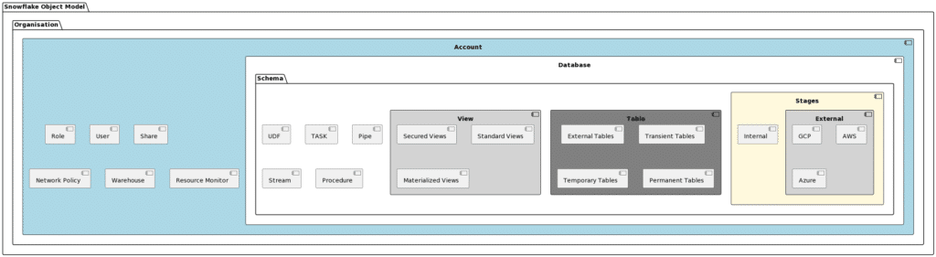
The Snowflake object model is a hierarchical framework that organizes and manages data within the Snowflake cloud data platform . An “object” itself refers to a logical container or structure that is used to either
Store data,
Organize data, or
Manage data.
From the top-level organization and account objects down to the granular elements like tables and views, the Snowflake object model provides a structured framework for data storage, access, and security. The following is a detailed overview of the key objects in the Snowflake object model and their respective functions.
Organisation
In Snowflake, an organisation is a top-level entity that groups together related accounts, providing a way to manage billing, usage, and access at a higher level.
Example: A multinational corporation might have a separate Snowflake organisation for each region it operates in, with individual accounts for each country.
Account
An account in Snowflake represents an independent environment with its own set of users, databases, and resources. It is the primary unit of access and billing.
Example: A retail company might have a Snowflake account dedicated to its e-commerce analytics, separate from other accounts used for different business functions.
Role
A role in Snowflake is a collection of permissions that define what actions a user or group of users can perform. Roles are used to enforce security and access control.
Example: A “Data Analyst” role might have permissions to query and view data in specific databases and schemas but not to modify or delete data.
User
A user in Snowflake is an individual or service that interacts with the platform, identified by a unique username. Users are assigned roles that determine their access and capabilities.
Example: A user named “john.doe” might be a data scientist with access to analytical tools and datasets within the Snowflake environment.
Share
A share in Snowflake is a mechanism for securely sharing data between different accounts or organisations. It allows for controlled access to specific objects without copying or moving the data.
Example: A company might create a share to provide its partner with read-only access to a specific dataset for collaboration purposes.
Network Policy
A network policy in Snowflake is a set of rules that define allowed IP addresses or ranges for accessing the Snowflake account, enhancing security by restricting access to authorized networks.
Example: A financial institution might configure a network policy to allow access to its Snowflake account only from its corporate network.
Warehouse
In Snowflake, a warehouse is a cluster of compute resources used for executing data processing tasks such as querying and loading data. Warehouses can be scaled up or down to manage performance and cost.
Example: A marketing team might use a small warehouse for routine reporting tasks and a larger warehouse for more intensive data analysis during campaign launches.
Resource Monitor
A resource monitor in Snowflake is a tool for tracking and controlling the consumption of compute resources. It can be used to set limits and alerts to prevent overspending.
Example: A company might set up a resource monitor to ensure that its monthly compute costs do not exceed a predetermined budget.
Database
A database in Snowflake is a collection of schemas and serves as the primary container for storing and organizing data. It is similar to a database in traditional relational database systems.
Example: A healthcare organization might have a database called “PatientRecords” that contains schemas for different types of medical data.
Schema
A schema in Snowflake is a logical grouping of database objects such as tables, views, and functions. It provides a way to organize and manage related objects within a database.
Example: In a “Sales” database, there might be a schema called “Transactions” that contains tables for sales orders, invoices, and payments.
UDF (User-Defined Function)
A UDF in Snowflake is a custom function created by users to perform specific operations or calculations that are not available as built-in functions.
Example: A retail company might create a UDF to calculate the total sales tax for an order based on different tax rates for each product category.
Task
A task in Snowflake is a scheduled object that automates the execution of SQL statements, including data loading, transformation, and other maintenance operations.
Example: A data engineering team might set up a task to automatically refresh a materialized view every night at midnight.
Pipe
A pipe in Snowflake is an object used for continuous data ingestion from external sources into Snowflake tables. It processes and loads streaming data in near real-time.
Example: A streaming service might use a pipe to ingest real-time user activity data into a Snowflake table for analysis.
Procedure
A procedure in Snowflake is a stored sequence of SQL statements that can be executed as a single unit. It is used to encapsulate complex business logic and automate repetitive tasks.
Example: A finance team might create a procedure to generate monthly financial reports by aggregating data from various sources and applying specific calculations.
Stages
In Snowflake, stages are objects used to stage data files before loading them into tables. They can be internal (managed by Snowflake) or external (located in cloud storage).
Example: A data integration process might use a stage to temporarily store CSV files before loading them into a Snowflake table for analysis.
External Stage
An external stage in Snowflake is a reference to a location in cloud storage (such as Amazon S3, Google Cloud Storage, or Azure Blob Storage) where data files are staged before loading.
Example: A company might use an external stage pointing to an Amazon S3 bucket to stage log files before loading them into Snowflake for analysis.
Internal Stage
An internal stage in Snowflake is a built-in storage location managed by Snowflake for staging data files before loading them into tables.
Example: An analytics team might use an internal stage to temporarily store JSON files before transforming and loading them into a Snowflake table for analysis.
Table
A table in Snowflake is a structured data object that stores data in rows and columns. Tables can be of different types, such as permanent, temporary, or external.
Example: A logistics company might have a permanent table called “Shipments” that stores detailed information about each shipment, including origin, destination, and status.
External Tables
External tables in Snowflake are tables that reference data stored in external stages, allowing for querying data directly from cloud storage without loading it into Snowflake.
Example: A data science team might use external tables to query large datasets stored in Amazon S3 without importing the data into Snowflake, saving storage costs.
Transient Tables
Transient tables in Snowflake are similar to permanent tables but with a shorter lifespan and lower storage costs. They are suitable for temporary or intermediate data.
Example: During a data transformation pipeline, a transient table might be used to store intermediate results that are needed for a short period before being discarded.
Temporary Tables
Temporary tables in Snowflake are session-specific tables that are automatically dropped at the end of the session. They are useful for temporary calculations or intermediate steps.
Example: In an ad-hoc analysis session, a data analyst might create a temporary table to store query results for further exploration without affecting the permanent dataset.
Permanent Tables
Permanent tables in Snowflake are tables that persist data indefinitely and are the default table type for long-term data storage.
Example: A financial institution might use permanent tables to store historical transaction data for compliance and reporting purposes.
View
A view in Snowflake is a virtual table that is defined by a SQL query. Views can be standard, secured, or materialized, each serving different purposes.
Example: A sales dashboard might use a view to present aggregated sales data by region and product category, based on a query that joins multiple underlying tables.
Secured Views
Secured views in Snowflake are views that enforce column-level security, ensuring that sensitive data is only visible to authorized users.
Example: In a multi-tenant application, a secured view might be used to ensure that each tenant can only see their own data, even though the underlying table contains data for all tenants.
Standard Views
Standard views in Snowflake are the default view type, providing a simple way to create a virtual table based on a SQL query without any additional security features.
Example: A marketing team might use a standard view to create a simplified representation of a complex query that combines customer.
Materialized Views
Materialized views in Snowflake are views that store the result set of the query physically, providing faster access to precomputed data.
Example: To speed up reporting on large datasets, a data warehouse might use materialized views to pre-aggregate daily sales data by store and product category.
In a previous article, we have already explored how to export data grom GA4 to BigQuery. In instances, where we want to migrate data from BigQuery to another platform like snowflake, BigQuery offers a few options.
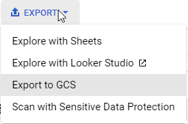
BigQuery Export options
Explore with Sheets:
Directly analyze and visualize your BigQuery data using Google Sheets.
Explore with Looker Studio:
Utilize Looker Studio (formerly Data Studio) for more advanced data exploration and interactive dashboard creation.
Export to GCS:
Save BigQuery datasets to Google Cloud Storage for storage or further processing with other tools.
Scan with Sensitive Data Protection:
Check your datasets for sensitive information before exporting, to ensure compliance and data privacy.
In out case, since we want to export the Google Analytics 4 data into Snowflake, we will need to first export it to Google Cloud Storage ( GCS ) . From this storage, we can then ingest data into Snowflake.
To understand the process flow, here is what we will be doing.
GA4 -> BigQuery -> Google Cloud Storage -> Snowfalke
A. Exporting from BigQuery to GCS
Deciding on Export Format
Before exporting, we want to decide on the format in which data will be exported for consumption. You can choose any of the format from CSV, JSON, Avro and Parquet depending on the use case. we will go with Parquet in this example. A brief comparison of these 4 data formats is given in the table below.
Feature
CSV
JSON
AVRO
Parquet
Data Structure
Flat
Hierarchical
Hierarchical
Columnar
Readability
High (Text-based)
High (Text-based)
Low (Binary)
Low (Binary)
File Size
Medium
Large
Small
Small
Performance
Low
Medium
High
Very High
Schema Evolution
Not Supported
Not Supported
Supported
Supported
Use Case
Simple analytics
Web APIs, Complex data
Long-term storage, Evolving schemas
Analytical queries, Large datasets
Compression
Low
Medium
High
Very High
Why Parquet?
Here’s a brief summary of why we chose Parquet for exporting GA4 data to BigQuery.
Columnar Efficiency
We benefit from Parquet’s columnar storage, optimizing our query execution by accessing only the necessary data.
Cost-Effective Storage
Our expenditure on data storage is minimized due to Parquet’s superior compression and encoding capabilities.
Support for Hierarchical Data
It supports our GA4 hierarchical data structures, ensuring the integrity of our analytical insights.
Seamless Integration
We utilize Snowflake’s native support for Parquet for straightforward data processing.
Schema Evolution Support
Since GA4 is in its early stage and new features keep on coming, we can gracefully manage changes in our data schema, avoiding costly downtime and data migrations.
Exporting Single Table
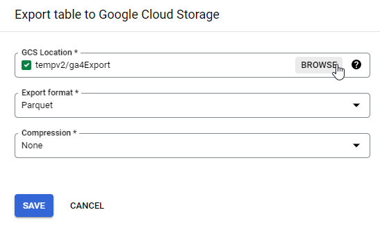
Clicking on the Export -> Export to GCS option will give us an option box to pick export format and compression. I have also specified a GCS storage location to store the export.
Exporting Multiple tables
Visual interface only allows export of a single table. Google Analytics 4, however, stores each day’s data separately as a single table. Therefore, we will have to find an alternative to visual export.
Shell script for Multiple table export
We can write a shell script which can export all our tables into our bucket. At a high level, we want our script to do the following :
Set Parameters: Define the dataset, table prefix, and GCS bucket.
List Tables: Use BigQuery to list all events_ tables in the dataset.
Export Tables: Loop through each table and export it to the designated GCS bucket as a Parquet file.
Here’s what the exact script looks like
#!/bin/bash

  # Define your dataset and table prefix

  DATASET="bigquery-public-data:ga4_obfuscated_sample_ecommerce"

  TABLE_PREFIX="events_"

  BUCKET_NAME="tempv2"

  # Get the list of tables using the bq ls command, filtering with grep for your table prefix

  TABLES=$(bq ls --max_results 1000 $DATASET | grep $TABLE_PREFIX | awk '{print $1}')

  # Loop through the tables and run the bq extract command on each one

  for TABLE in $TABLES

  do

      bq extract --destination_format=PARQUET $DATASET.$TABLE gs://$BUCKET_NAME/${TABLE}.parquet

   done
Save the script and give it a name. I named it export_tables.sh. Change the script mode to chmod +x.
Execute the shell script with ./export_tables.sh
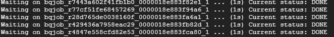
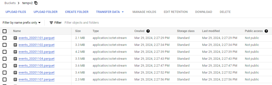
If everything works out correctly, you will start to see output :
You can check whether data has been exported by inspecting the contents of the storage bucket.
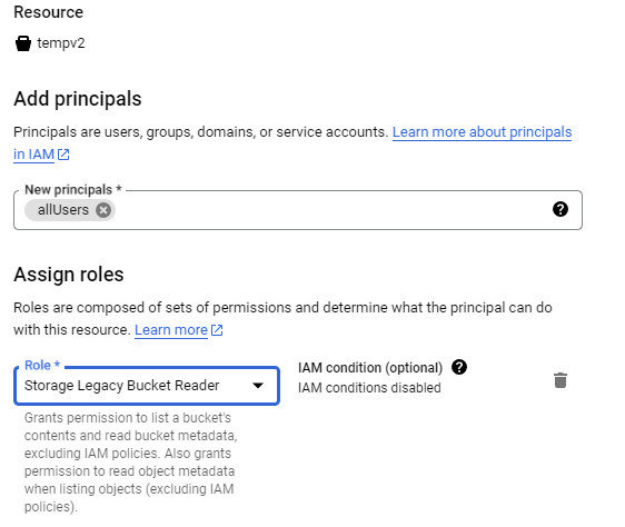
Allow appropriate access , so that you can read the data in snowflake. You can do this by opening the bucket > Permissions and then click on Grand Access.
In this example, I have granted access to allUsers. This will make the bucket readable publicly.
To ingest the data from Google cloud storage into snowflake, we will create storage integration between GCS and snowflake and then create an external stage. Storage integration streamlines the authentication flow between GCS and Snowflake. External stage, allows snowflake database to ingest the data.
Top of Form
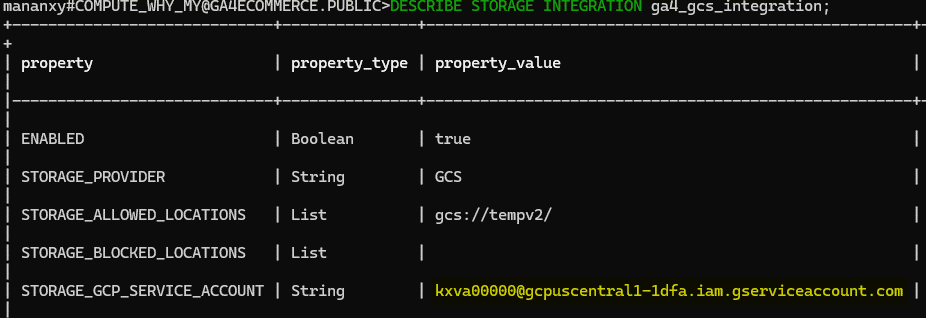
B. Create Storage Integration in Snowflake
Storage integration in snowflake will create a temporary service account. We will then provision access to that temporary account from GCP.
Log into Snowflake: Open the Snowflake Web UI and switch to the role with privileges to create storage integrations (e.g., ACCOUNTADMIN).
Snowflake will automatically create a GCP service account . We will then go back to Google Cloud to provision necessary access to this service account.
Navigate to GCS: Open the Google Cloud Console, go to your GCS bucket’s permissions page.
Add a New Member: Use the STORAGE_GCP_SERVICE_ACCOUNT value as the new member’s identity.
Assign Roles: Grant roles such as Storage Object Viewer for read access
C. Create External Stage in Snowflake
External stage will allow snowflake database to ingest data from external source of GCP.
Define the File Format (if not already defined):
CREATE OR REPLACE FILE FORMAT my_parquet_format
TYPE = ‘PARQUET’;
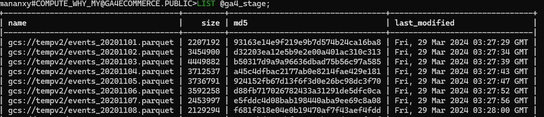
Create External Stage
CREATE OR REPLACE STAGE my_external_stage
URL = ‘gcs://tempv2/’
STORAGE_INTEGRATION = gcs_storage_integration
FILE_FORMAT = my_parquet_format;
Verify the external stage with LIST command, you can see the output
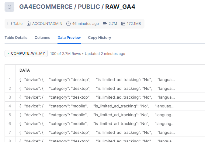
Create table to load data into
We will create a table , so that we can load data from the stage into the table.
create table raw_ga4 (
data VARIANT
)
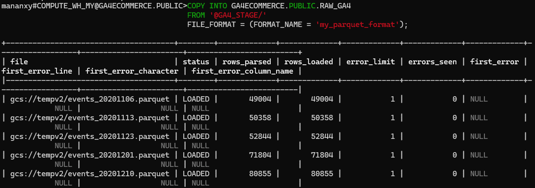
Load data from stage
Finally, we can load data from external stage into snowflake database table using COPY INTO command.
There are 2 primary ways that we can ingest data into snowflake database.
With an upfront Schema
Without an upfront Schema
In this case, we will ingest the data without having an upfront schema.
D. Loading data without Schema
Snowflake provides a ‘VARIANT’ data type. It is used to store sem-structured data such as SON, Avro or Parquet etc. Its useful because it allows you to ingest and store data without needing to define a schema upfront. The VARIANT column can hold structured and semi-structured data in the same table, enabling you to flexibly query the data using standard SQL alongside Snowflake’s powerful semi-structured data functions.
Therefore, in Step4 , we create a simple table with VARIANT column of data.
To load the data into our raw_ga4 table, we use the following command.