Evaluating Azure ML Regression Results.
In the earlier article, we used Azure ML Designer to build a regression model. The final output of the regression model is few metrics which we use to understand how good our regression model is.
There are two steps of interest in evaluating the efficiency of the model. The score model step predicts the price, and evaluate model step finds the difference between prediction and actual price which was already available in the test dataset.
| Azure ML Step |
Function |
Dataset |
| Train Model |
Find mathematical relationship(model) between input data and price |
Training dataset |
| Score Model |
Predict prices based on the Training model |
Testing dataset.
Added 1 more column of forecasted price. |
| Evaluate Model |
Calculate the difference between prediction and the actual price |
Testing data set. |
Score Model
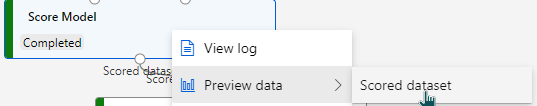
Before going to evaluation, it is pertinent to investigate the output of Score Model and what has been scored.
Understanding Scoring
When we were training our model, we selected the Label column as Price.
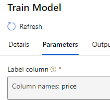
Training model for label price means in simple terms is :
Using 25 other columns in the data, find what is the best combination of values, which can predict the value of our Label column (price)
Scoring model
- Used training model to predict the value of price
- Used test dataset and provide a predicted value of price
Therefore, after scoring, we will have an extra column added at the end of the scored data set, called Scored Labels. It looks like this in preview
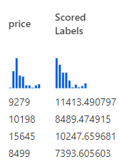
This new column “Scored Labels” is the predicted price. We can use this column to calculate the difference between the actual price which was available in the test data set and how the predicted price (Scored Labels) is
The lower the difference, the better the model is. Hence, we will use the difference as a measure to evaluate the model. There are several metrics which we can use to evaluate the difference.
Evaluate Model
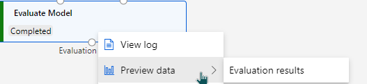
We can investigate these metrics by right clicking on Evaluate Model > Preview data > Evaluation results
The following metrics are reported:
Both Mean Absolute Error and Root Mean Square error are averages of errors between actual values and predicted values.
I will take the first two rows of the scored dataset to explain how these metrics evaluate the model.
| make |
Wheel-base |
length |
width |
…. |
Price |
Predicted price
(Scored Label) |
| Mitsubishi |
96.3 |
172.4 |
65.4 |
… |
9279 |
11413.49 |
| Subaru |
97 |
173.5 |
65.4 |
… |
10198 |
8489.47 |
Absolute Errors
Mean Absolute Error
Evaluates the model by taking the average magnitude of errors in predicted values. A lower value is better
Using the table above, MAE will be calculated as :
| Price |
Predicted price
(Scored Label) |
Error =
Prediction – Price |
Magnitude of error |
Average of error |
| 9279 |
11413.49 |
2,134.49 |
2,134.49 |
854.76 |
| 10198 |
8489.47 |
-1,708.53 |
1,708.53 |
854.76 for the above 2 rows is the average error. Let’s assume there was another model whose MAE will be 500.12. If we were comparing two models
Model 1 : 854.76
Model 2 : 500.12
In this case, model 2 will be more efficient than Model 1 as its average absolute error is less.
Root Mean Squared error
RMSE also measures average magnitude of the error. A lower value is better. However, differs from Mean Absolute Error in two ways :
- it creates a single value that summarized the error
- Errors are squared before they are averaged, hence it gives relatively high weight to large errors. E.g., if we had 2 error values of 2 & 10, squaring them would make them 4 and 100 respectively. This means that larger values get disproportionately large weightage.
This means RMSE should be more useful when large errors are particularly undesirable.
Using the table above, RMSE will be calculated as :
| Price |
Predicted price
(Scored Label) |
Error =
Prediction – Price |
Square of Error |
Average of Sq. Error |
Square root. |
| 9279 |
11413.49 |
2,134.49 |
4,556,047.56 |
3,737,561.16 |
|
| 10198 |
8489.47 |
-1,708.53 |
2,919,074.76 |
Relative Errors
To calculate relative error, we first need to calculate the absolute error. Relative error expresses how large the absolute error is compared with the total object we are measuring.
Relative Error = Absolute Error / Known Value
Relative error is expressed as a fraction, or multiplied by 100 to be expressed as a percent.
Relative Squared error
Relative squared error compares absolute error relative to what it would have been if a simple predictor had been used.
This simple predictor is average of actual values.
Example :
In the Automobile price prediction, we have an absolute error of our model which is Total Squared Error.
Instead of using our model to predict the price, if we just take an average of the “price” column. Then find squared error based on this simple average. It will give us a relative benchmark to evaluate our original error with.
Therefore, the relative square error will be :
Relative Squared Error = Total Squared Error / Total Squared Error of simple predictor
Using the two-row example to calculate RSE :
Calculate Sum of Squared based on Simple Predictor of Average
| Price |
Average of Price
(New Scored Label) |
Error =
Prediction – Price |
Sum of Squared |
| 9279 |
9,738.5 |
459.5 |
|
| 10198 |
9,738.5 |
459.5 |
|
Mathematically relative squared error, Ei of an individual model i is evaluated by :

Relative Absolute Error
RAE compares a mean error to errors predicted by a trivial or naïve model. A good forecasting model will produce a ratio close to zero. A poor model will produce a ratio greater than 1.
Relative Absolute Error = Total Absolute Error / Total Absolute Error of simple predictor
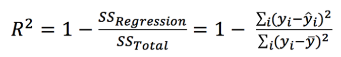
Coefficient of determination
The coefficient of determination represents the proportion of variance for a dependent variable (Prediction) that’s explained by an independent variable (attribute used to predict).
In contrast with co-relation which explains the strength of the relationship between independent and dependent variables, the Coefficient of determination explains to what extent variance of one variable explains the variance of the second variable.
R (Correlation) (source: http://www.mathsisfun.com/data/correlation.html)
Azure machine learning studio provides an easy-to-use interface for data scientists and developers to build train and productionise machine learning models. Another major benefit it provides is the ease of collaboration and
In this article, we will explore how to solve a machine learning problem with Azure Machine Learning Designer.
Defining the Problem
To solve the problem via Azure ML Studio. We need to do the following steps
- Create a Pipeline,
- Set pipeline’s compute target.
- Importing Data
- Transforming Data
- Train the Model
- Testing the Model
- Evaluate the Model
Creating pipeline using ML Designer
Azure machine learning pipelines are workflows of executable steps that enable users to complete Machine Learning workflows. Executable steps in azure pipelines include data import, transformation, feature engineering, model training, model optimisation, deployment etc.
There are 3 ways of creating pipelines in Azure Machine learning Studio
- Using Code ( Python SDK )
- Using Auto ML
- Using ML Designer.
- When we login to Azure ML Studio , we see the following options.
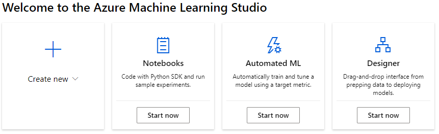
- Click on Designer (Start Now) to create a new Pipeline.
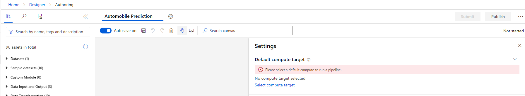
By default it’s given a name based on today’s date. I have changed it to Automobile Prediction.
Setting Compute Target
A compute target is an instance of Azure virtual machine which will be used to provide processing power for our pipeline execution.
Default compute target will be used for entire pipeline, we can also use separate compute targets for individual steps of execution.
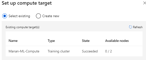
I created a compute instance earlier, so I can select existing
Importing Data
We can import the data from several sources. For this article, I will use sample datasets provided by Azure.
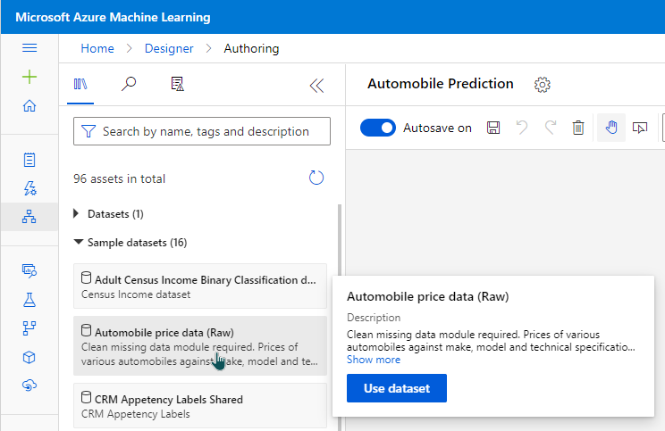
To explore what is in the data set, we can click on the data set and go to preview data.
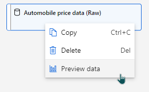
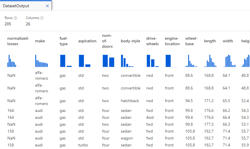
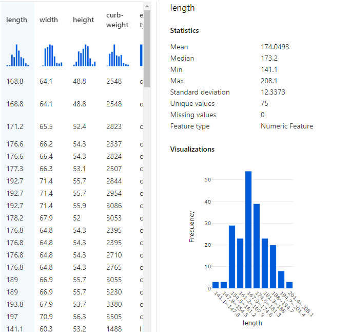
This provides us a sneak-preview of what’s included in the data. E.g. there are 205 rows, 26 columns. Clicking on each column provides key statistics about data in that specific column. E.g. If I click on length column, I get a histogram showing the frequency of length values and various other statistics about it.
Transform Data
The data preview feature is helpful in understanding the columns and transforming data for any characteristics necessary to run our model.
Exclude a column
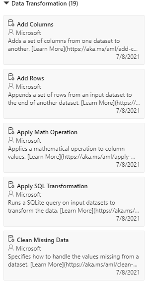
The data transformation section on left side menu provides several commonly used data transformation operations.
I want to remove the column normalized-losses
So, I can drag and drop “Select Columns in Dataset”
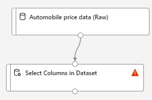
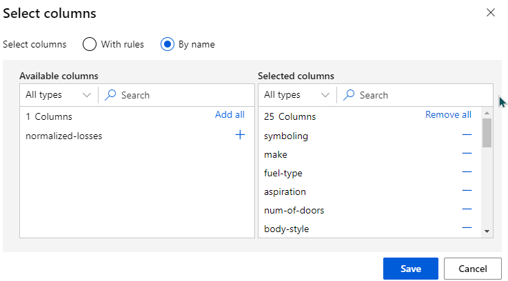
When I go to the details of “Select Columns in Dataset” , I can then select all columns other than normalized losses
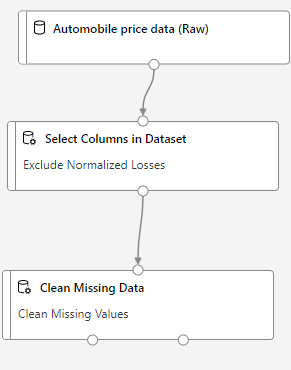
Clean Missing Data
After removing the normalized-losses columns, our data still has empty values. To clean the missing data. I can use Clean Missing Data module from left side menu. So that our worspace looks like
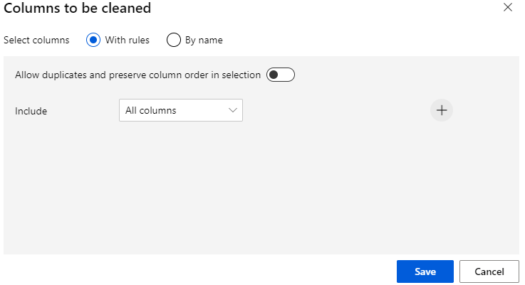
Going into details of Cleaning missing data, I can select Alll columns.
Training the Model
I want to divide my dataset rows into
- Training rows (training dataset)
- Testing rows (testing dataset)
I can use Split Data Module from left side menu, so that my pipeline will now look like :
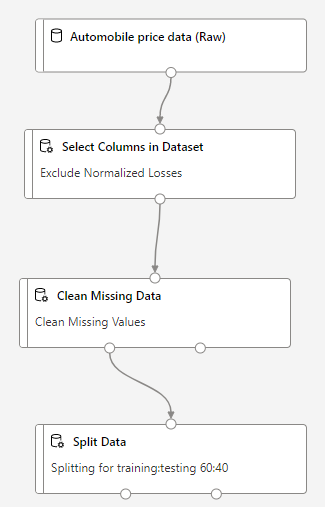
The Split Data module has 2 outputs. The left outputwill connect to Train Model and Right output will connect to Test Data.
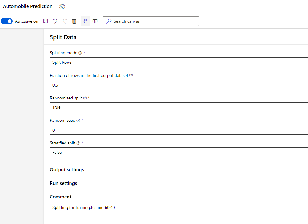
In the details of Split Data module, I can choose the ratio with which I want to split the data across training and testing.
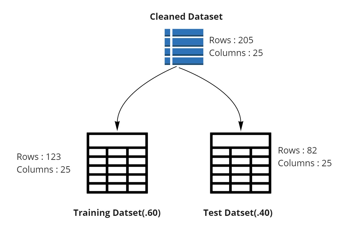
In summary, we cleaned the dataset and then divided it into two separate one as shown in the image below.
Training the Model
To train any model, we need to have.
- The model
- The data on which model is to be trained.
In our case, we want to predict automobile prices using Linear Regression Model. The training data for Linear Regression Model is the one which we have split from our overall data.
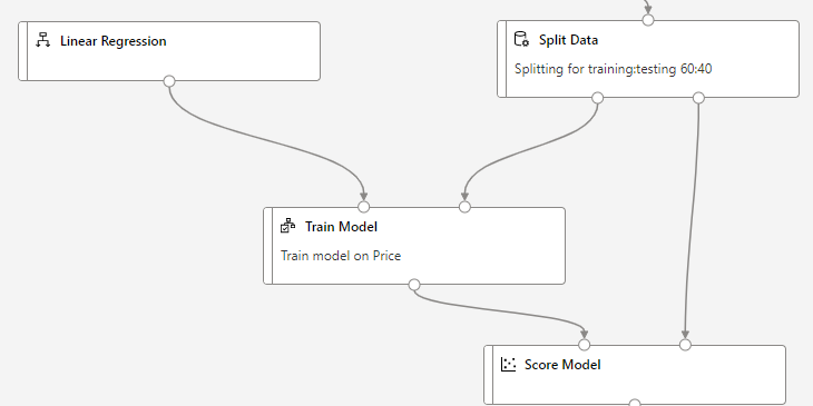
Therefore, we can train our model by combination of Linear Regression module and Train Model module from left side menu.
The Train Model module requires a label to train the model for. A label in this case is independent variable? with the help of which we can find the dependent variable.
[From y = mx + c , a label is X ]
Testing the Model
In Split Data step above, we used only 60 % of our data for training the model. We left remaining 40% of the data for testing. We can setup the testing now by using Score Model module.
Score Model module will need two input.
- What needs to be tested (output of our trained model)
- With what to test (test data from split)
This will look like:
Evaluating the Model
Now we want to see how our model scored when compared against the test dataset. We can use Evaluate Model module and connect Score Model module to it.
This will finish our pipeline creation. We now need to submit it.
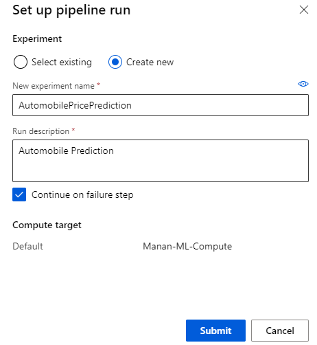
Pipeline Submission
Pipeline submission will create an experiment name and compute target.
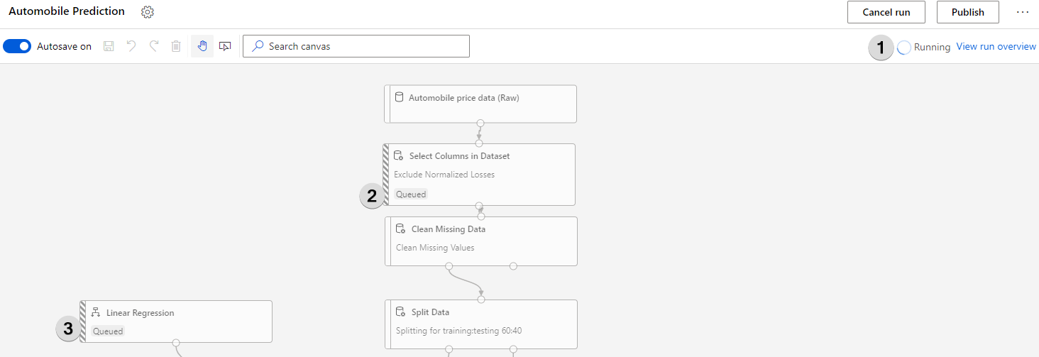
Understanding the Predictions
Azure ML takes a bit of time especially if the experiment is run for the first time. You can view the progress by looking at the “Running” status (1) or by looking at what’s the status of each individual module ( 2, 3).
Once the model finishes it run, right-click on Score Model and select Visualize > Scored dataset
In the Scored Labels column, you can see the predicted prices.
Understanding Models efficiency
We can use Evaluate Model to see the efficiency of the trained mode.
Right click Evaluate Model -> Visualize -> Evaluation Results
The following statistics are available.
- Mean Absolute Error
- Root Mean Squared Error
- Relative Absolute Error
- Relative Squared Error
- Coefficient Determination
Azure machine learning pipelines are workflows of executable steps that enable users to complete Machine Learning workflows. Executable steps in azure pipelines include data import, transformation, feature engineering, model training, model optimisation, deployment etc.
Benefits of Pipeline:
- Multiple teams can own and iterate on individual steps which increases collaboration.
- By dividing execution into distinct steps, you can configure individual compute targets and thus provide parallel execution.
- Running in pipelines improves execution speed.
- Pipelines provide cost improvements.
- You can run and scale steps individually on different compute targets.
- The modularity of code allows great reusability.
Creating a pipeline in Azure
We can create a pipeline either by using Machine learning Designer or by using python programming
Creating pipeline using Python
1. Loading the workspace configuration
from azureml.core import Workspace

ws = Workspace.from_config()
2. Creating training cluster as a compute target to execute our pipeline step
from azureml.core.compute import ComputeTarget, AmlCompute

compute_config = AmlCompute.provisioning_configuration(

vm_size='STANDARD_D2_V2', max_nodes=4)

cpu_cluster = ComputeTarget.create(ws, cpu_cluster_name, compute_config)

cpu_cluster.wait_for_completion(show_output=True)
3. Defining estimator which provides required configuration for a target ML framework:
from azureml.train.estimator import Estimator

estimator = Estimator(entry_script='train.py',

compute_target=cpu_cluster, conda_packages=['tensorflow'])
4. Configuring the estimator step
from azureml.pipeline.steps import EstimatorStep

step = EstimatorStep(name="CNN_Train",

estimator=estimator, compute_target=cpu_cluster)
5. Defining and executing a pipeline :
from azureml.pipeline.core import Pipeline

pipeline = Pipeline(ws, steps=[step])
Pipeline is defined simply through a series of steps and is linked to a workspace.
6. Validating pipeline to check
7. All steps are validated. We can now submit it as an experiment to workspace.
from azureml.core import Experiment

exp = Experiment(ws, "simple-pipeline")

run = exp.submit(pipeline)

run.wait_for_completion(show_output=True)
Creating pipeline using ML Designer
We have covered pipeline creation using Azure Machine Learning Designer in another article in detail.