Loading Data from Kaggle to Amazon S3 Bucket

Loading data from kaggle directly into S3 is a two step process. In first step we configure Kaggle to be able to download. And in second step, we extract data from Kaggle into S3 bucket.

Get data from Kaggle

To get data from kaggle, we setup Kaggle command line tool and then generate an API token to get the data.

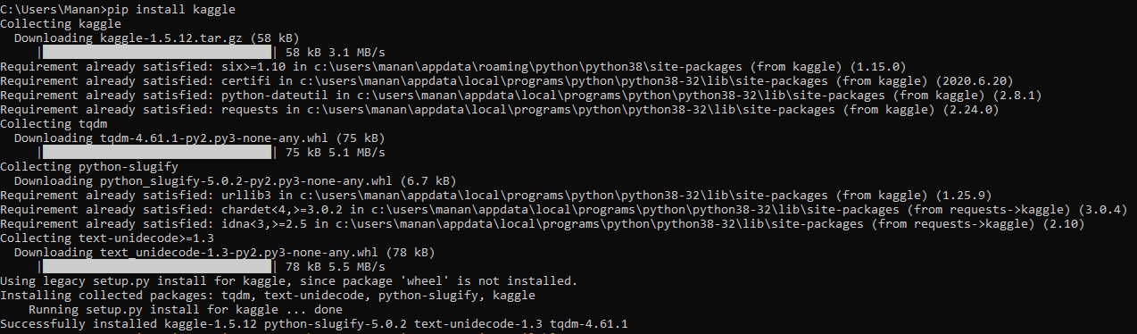
Setup Kaggle Command Line

To get data from Kaggle, we will install kaggle-cli.

pip install kaggle

Create API tokens

From top right, click on your account name and then click on Account

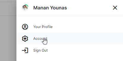
Account page has a panel for creating new Api token.

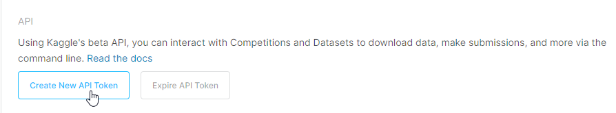
It will download kaggle.json which we can then use as a token. Move this file to Kaggle’s Environment folder. By default its in user’s home directory /.kaggle/

Download data on local

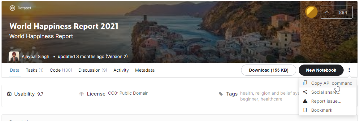
To demonstrate, I am using this dataset from Kaggle.

From the three dots on the right side, select the Copy API command.

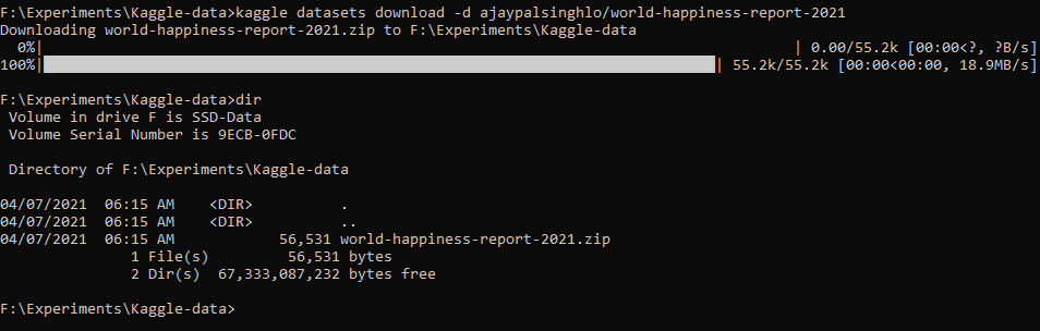
[su_box title=”Copy data” style=”glass” radius=”1″]kaggle datasets download -d ajaypalsinghlo/world-happiness-report-2021[/su_box]

This will download the file on your local desktop.

Copy data to S3

Setup AWS Command Line

To copy data from local desktop to AWS s3 bucket, AWS provides CLI tools. To use AWS CLI tools, we first need to generate aws access credentials. This can be done from AWS web console.

Generate S3 AWS secret

In the AWS S3 interface. Select IAM -> Users from services.

Click on Add User.

Check Programmatic access.

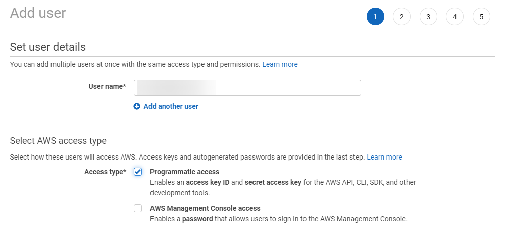
It will generate an access key id and secret access key.

Configure Keys in local system

To check AWS key configuration, type :

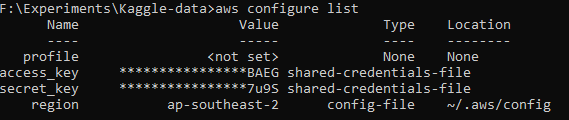
aws configure list

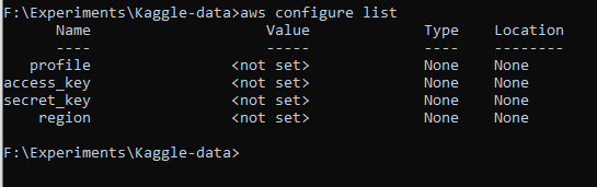
Use aws configure command to enter the key and secret from the previous step.

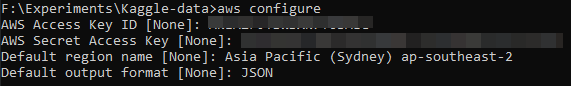
Succesful configuration will result in a configuration list that looks like the following :

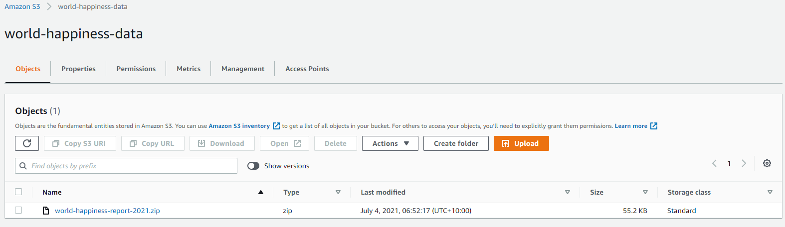
Create S3 Bucket

In the AWS console, select service S3 and click on Create Bucket.

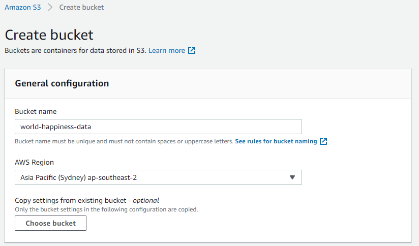
URI to access the bucket is not displayed in the console. However, it’s s3://bucket name. In our case, it will be s3://world-happiness-data

Copy data from local to S3

Now that bucket is created and our CLI is configured, we can run the copy command.

aws s3 cp world-happiness-report-2021.zip s3://world-happiness-data

verifying upload

We can verify the upload by going to Amazon AWS console > S3 > Bucket name

Correlation Coefficient – Simplistic explanation

What is Correlation Coefficient

Correlation means a mutual relationship or connection between two or more things (variables). The correlation coefficient is a numeric measure to quantify this relationship. The coefficient describes two aspects of a relationship.

Strength of the relationship
Direction of the relationship.

Correlation is used for predicting the relationship between two variables. It is also used for concurrent validity ( correlation between a new measure and an established measure). One more use of correlation is in reliability testing, e.g. Test-retest reliability (measure consistent).

Strength of relationship

For the strength of the relationship, the value ranges from 0 to 1. A perfectly strong relationship between variables will be 1, whereas no relationship between two variables will be 0. Values in the vicinity of 0.5 ( middle of 0 & 1 will represent a medium correlation).

Perfect Correlation

The perfect correlation will have a value of 1. The Scatter plot below shows a perfect correlation, as one variable increases, the other variable increases as well.

Strong & Weak Correlation

A correlation will mean stronger relationship between two variables under study. There is no rule for determining what’s considered Strong, medium or week. The interpretation of coefficient depends on subject of study.

In one area of study 0.4 and above could be considered as relatively strong, whereas in another subject 0.4 can be considered relatively week, and only vales of 0.75 and up are considered as strong correlation.

The scatter below has a correlation value of 0.944. It’s direction is positive. It represent a very strong correlation indicating that as X increase, Y will strongly increase with it.

The scatterplot below has a correlation value of 0.0478. Its direction is positive, however, it’s a weak correlation.

Direction of relationship

The direction of the relationship indicates an inverse relationship between the variables. An increase in one variable is associated with a decrease in the other variable. An example of negative correlation will be Boyle’s law as the volume of a container increases, the pressure of gas decreases.

The Scatter plot below shows a perfect correlation of (-1), as one variable increases, the other variable decreases with it.

Methods of calculating Correlation Coefficient

There are multiple methods for calculating correlation coefficient e.g.

Pearson’s method
Kendal’s methods
Pearson’s methods.

For this article, I will focus on Pearson’s correlation coefficient.

Pearson’s Correlation Coefficient

Let’s begin by looking at the formulae for Pearson’s Correlation coefficient

r = \frac{{}\sum_{i=1}^{n} (x_i - \overline{x})(y_i - \overline{y})} {\sqrt{\sum_{i=1}^{n} (x_i - \overline{x})^2(y_i - \overline{y})^2}}

Where,

$x_i$ is the individual value of the x

$\overline{y}]$ is the mean of all x values

Numerator in Pearson’s equation

r = \frac{{}\sum_{i=1}^{n} (x_i - \overline{x})(y_i - \overline{y})} {}

All we are doing here is finding the error by subtracting the predicted x and y values from their respective mean. For examples, $(x_i - \overline{x})$ finds the difference of each x value from it’s mean. We repeat it for each value of $y_i$ and sum the resultant number. In a more statistical language, we are essentially normalizing the chart around the mean.

Denominator in Pearson’s equation

r = \frac{} {\sqrt{\sum_{i=1}^{n} (x_i - \overline{x})^2(y_i - \overline{y})^2}}

$(x_i - \overline{x})^2$ is the sum of errors squared. It calculated the distance between individual predicted x values and mean of all x values. Similarly

Loading data in Snowflake

Any relational database for example ( MYSQL, POSTGRESQL) can only support structured data in the forms of rows and columns. Snowflake, however, can support multiple types of data loads.

Snowflake Supported Formats

Supported File	Encoding
Delimited files (CSV, TSV, etc.)	UTF-8
JSON	UTF-8
Avro	UTF-8
ORC	UTF-8
Parquet	UTF-8
XML

Concept of stages

Internal Stages

Snowflake has the following stage types. Data can be uploaded to any of the internal stage type from local file system using PUT command.

Snowflake Internal Stages

Stage	Description
User	A user stage is allocated to each user for storing files. This stage type is designed to store files that are staged and managed by a single user but can be loaded into multiple tables. User stages cannot be altered or dropped.
Table	A table stage is available for each table created in Snowflake. This stage type is designed to store files that are staged and managed by one or more users but only loaded into a single table. Table stages cannot be altered or dropped.
Named	A named internal stage is a database object created in a schema. This stage type can store files that are staged and managed by one or more users and loaded into one or more tables. Because named stages are database objects, the ability to create, modify, use, or drop them can be controlled using security access control privileges. Create stages using the CREATE STAGE command.

External Stages

Snowflake supports direct data load from cloud platforms. The table below summarizes the supported platforms.

Snowflake Platforms for Data Load

Supported Platform	Loading Stages
Local environment	Files are first staged in a Snowflake stage, then loaded into a table.
Amazon S3	Files can be loaded directly from any user-supplied S3 bucket.
Google Cloud Storage	Files can be loaded directly from any user-supplied Cloud Storage container.
Microsoft Azure	Files can be loaded directly from any user-supplied Azure container.

Loading data from Amazon AWS

Creating an S3 Stage

An S3(external) stage is a reference to a location in the snowflake platform where data files are stored before they are loaded into a table.

Loading all files within the folder:

If the path ends with /, all of the objects in the S3 folders are loaded in the stage

Loading data from a file

If specific file path is given, it loads data from file into the stage. The example below loads CSV data into an S3 stage.

To create a stage, Select the database > Click on Stages Tab -> Click on Create

This loads a create stage interface where we can specify file information to load data from

CREATE STAGE “ANALYTICS_DEMO_DATA_2″.”PUBLIC”.My_First_External_Stage URL = ‘s3://world-happiness-data/world-happiness-report-2021.csv’ CREDENTIALS = (AWS_KEY_ID = ‘AKIAZFJYSWSXK7Y6BAEG’ AWS_SECRET_KEY = ‘****************************************’);

Viewing Stages:

We can view available stages in our database using the following command.

Show stages;

This shows the stage we created in previous step

Copying data from Stage

Now that the data is loaded in the Snowflake stage. We can load it on our table.

copy into “ANALYTICS_DEMO_DATA_2″.”PUBLIC”.”S3DATA” from @MY_First_External_Stage;

A select statement to confirm loading shows that data is successfully loaded from the stage into our table.

Bulk vs continuous loading

External tables (Data Lake)

Snowflake Basic Operations

What is snowflake?

Snowflake is a data warehouse platform that pitches the native cloud ( or cloud-first ) approach as its primary value proposition. let’s learn about snowflake by going hands-on in few basic operations in snowflake.

Creating Database in snowflake

Creating a database in snowflake is fairly easy and standard. There are two approaches of doing it.

Graphical Interface

Clicking on the Databases tabs from the main menu loads the database panel. Click on create to create a database.

SQL Command line

The other way of creating a database in snowflake is via the command line. For that, click on the Worksheets tab. Worksheet in snowflake is an interface for viewing all data objects. Click on + sign to create a new worksheet if you prefer, or continue to work in the default worksheet.

1. The left side of worksheet lists all the database objects.

2. SQL space is where we can write SQL queries ( in this case to create a database)

3. On top right, it gives basic information about role, instance type and the current database selected.

Coming back to query for creating database.

Write query in the worksheet.
Results show up at the bottom pane
Refresh the left pane and we have our database ready.

[su_box title=”Creating Database with SQL” style=”glass” radius=”1″]CREATE DATABASE “ANALYTICS_DEMO_DATA_2”;[/su_box]

Creating Schema in snowflake

A schema is a logical grouping of database objects ( tables, views, etc. ). In contrast, a database is a logical grouping of schemas. Each schema belongs to a single database.

To create schema in snowflake, go to the Databases tab. Click on the database name for which you want to create the schema. Then click on Schemas sub-menu.

Select database for which you want to create the schema
Click on Schemas sub-menu
Click on Create button
Enter schema name

SQL alternative for schema creation will be.

[su_box title=”Creating Schema with SQL” style=”glass” radius=”1″]CREATE SCHEMA “ANALYTICS_DEMO_DATA”.”DEMO_SCHEMA”;[/su_box]

Creating a table in snowflake database

To create a table in snowflake via Graphical interface.

Select the database you want to create a table in, from the Databases menu.
Tables sub-menu is selected by default. Click on + Create.
Enter the table name.
Add a column ( you need atleast 1 column to create the table ).

The SQL way of creating a table will be.

[su_box title=”Creating Table with SQL” style=”glass” radius=”1″]CREATE TABLE “ANALYTICS_DEMO_DATA_2″.”PUBLIC”.”MY_FIRST_TABLE” (“C1” STRING) COMMENT = ‘Hello World Table’;[/su_box]

Creating views in snowflake database

To create a view in snowflake via Graphical interface.

Select the database you want to create a table in, from the Databases menu.
Select the views sub-menu. Click on + Create icon.
Enter the view name.
Enter the view definition.

SQL way of creating a way in snowflake would be :

[su_box title=”Creating views with SQL” style=”glass” radius=”1″]CREATE VIEW “ANALYTICS_DEMO_DATA_2″.”PUBLIC”.My_First_view AS Select C1 from My_First_Table;[/su_box]

Previewing data in snowflake

We can preview the data in snowflake from the worksheet menu.

From the left side database object menu, select the table to preview
Click on the preview data button
Data preview will show in bottom pane

I have selected a sample Citibank database and trips table in it for preview.

This was a high-level overview of getting started with snowflake. We’ll look into how to load data in snowflake and the concept of stages.

Regression Analysis

What is Regression Analysis

Regression analysis is a process to find a relationship between two or more variables.

A variable can represent data from any word, event, occurrence, phenomenon, etc.

For example, say we want to find whether there’s any relationship between cold weather and coffee sales in Melbourne. First variable is cold weather, the second variable is increase in coffee sales.

We can use Regression Analysis to find out

Whether there’s any relationship between cold weather and coffee sales.
What is the extent of this relationship? Does cold weather double coffee sales or half it?

Objectives of Regression Analysis

The primary objective of regression analysis is to:

Determine the relationship between two variables.
Predict future results based on existing knowledge.

Digital Analytics Use Cases of Regression Analysis

Regression analysis is frequently used in web analytics, digital marketing analytics and other machine learning algorithms. Few examples would be:

Understanding the impact of Digital marketing channels on Sales. For example, If you are using digital marketing and TV ads. You can establish a relationship between your online & offline channels on your net sales.
If your website offers paid services, you can use regression analysis to predict whether a customer is likely to leave your paid service. Hence you can take proactive action to stop the customer from churning.

Methods of Regression Analysis

There are several methods used for regression depending on the use case. For example, linear regression, logistic regression, and mixed regression.

Linear Regression

We will focus on linear regression as its simplest to understand

1.Data Representation on Graph

Let’s say we want to find out a relationship between advertising cost and online sales. We have data for 5 campaigns.

Digital Ad Dollars (Million)	Monthly E-commerce sale (Million)
5	20
20	75
10	46
25	80
30	100

To get a visual understanding of our data. Let’s put them on a scatter plot

(A scatter is a graphical way of representing the relationship between two variables)

Our task is to establish a relationship so that we can use that relationship to predict future sales. In our example, we want to find out what would be our sale if we spend 40 million dollars or 45 million dollars.

Digital Ad Dollars (Million)	Monthly E-commerce sale (Million)
35	?
40	?

2.Assuming straight lines

Let’s assume that there’s a straight line running through the graph that predicts the future value with 100% accuracy. If we could predict the data accurately, the values for X-axis 35 and 40 will land precisely on our perfect assumption line. However, that’s an unknown.

If we could visually draw assumption lines to “predict” relationship, then we can theoretically draw unlimited lines, one of them would be perfect. We cannot know which one.

Linear regression forecasts the value of unknown data points ( in our example, 35 & 40) by finding the best fit line through the points. The best-fitting line is called a regression line.

3.Best Fit line – Regression line

A best-fit line should minimize the error between values forecasted by it and the actual ( unknown ) values.

Different methods are available for finding the best fit line. Few of the methods are

Generalized method of moments ( GMM)
Maximum Likelihood estimation ( ML)
Ordinary Least Square method ( OLS)

Most used method is ordinary least square method.

Ordinary Least Square method

Least square method was officially discovered & published by Adrien-Marie in 1805. Ordinary least square method works by minimizing the sum of squares of the known ( observed) values and those predicted by the linear function.

If we could plot n random lines through the points and calculate the sum of residuals ( distance from observed value to the value on our assumed line), each line will have multiple error values( one for each data point) . Summing up those values and then squaring them will give us a single number. Let’s call it sum of squares. If we drew 10 lines, we will have 10 different sum of squares. Our task is to find the value with the least sum of squares.

Mathematically sum of squares errors can be written as

Where

: is the actual value

: is the estimated (or predicted) Y value

The predicted value can be calculated using a simple line equation

Replacing the value of estimated ( or predicted ) Y value in the sum of square error equation.

From here, we can use calculus to differentiate this equation with respect to the first regression coefficient and set it to zero, then differentiate with respect to other regression coefficient and set it to zero, thus deriving sample regression function.

SRF (Sample Regression Function) :