Facebook use auctions to determine which ads to show to the user. This is similar to how google price its ads. In this article we will explore how facebook’s Ad auction system works.
Facebook Ad Auction system has two goals :
Create value for advertisers ( maximise return on investment)
Provide positive user experience ( show relative ads )
Each time an auction takes place, facebook’s algorithm decide which ad to show based on Total Value for each Ad
Total Value = Advertiser bid * Estimated action rate + Ad quality
Lets go into each of these factors individually.
Advertiser bid :
Bid is the price that you are willing to pay for an Ad in dollars. This Ad bid can be either specificed manually or you can let facebook decide the best price. The important factor to note is that highest bid price does not guarantee that Ad will always be served to the audience your target audience. Final Ad display will always be calculated by Total Value formulae.
Estimated action rate :
Estimated action rate is based on Ad relevance. If an Ad is more aligned with user’s interest, it gets higher score. If same ad is less aligned, it gets lower score. We can understand it with an example.
Ad
Audience Interest
Relevance Score
(hypothetical score out of 1)
Estimated action rate
Creative 1
Health & wellbeing
0.8
High
Creative 1
Fast food & desserts
0.1
Low
The scoring method used in the example above is arbitrary and only used for illustration purpose only.
While facebook does not explicitly lists the factors making up estimated action rate, following factors are indicative of what makes up estimated action rate.
Relevant campaign objectives
Relevant audience
High quality creatives
Historical conversion probability
Ad Quality :
Ad quality is determined by several factors. The actual factors are not explicitly given by facebook. However, the objective of Ad quality is that to serve relevant Ads to right audiences. The following factors contribute to Ad Quality score :
CTR ( click-through rate of the ad)
Ads relevancy score
Crowdsourced Feedback of the Ad ( Ads hidden , reported bad)
Text to Image ratio
Landing Page experience
Landing Page speed
Authenticity of landing page
Authenticity of business
Popup, ads or other contents which can be detrimental for user experience
Expected conversion rate
Historical conversion rate
Weightage of factors ?
Facebook does not provide the weightage of each factor in the Total Value formulae. In an ideal world, advertiser’s would have the formulae with weigtahges e.g. if x,y and z are the weigthages then formulae would be like:
Total Value = (x)Advertiser bid * (y)Estimated action rate + (z)Ad quality
However, these weightages remain unknown to the advertisers. Only facebook knows the recipe of the secret sauce of x,y & z.
Facebook Charging Model:
Facebook has 3 charging models which it uses for billing its advertisers.
CPM billing
Link click billing
Action based billing
1. CPM billing:
Since facebook is primarily a display based Ad platform. It’s most dominant biling format is CPM. CPM stands for cost per Mile ( 1000). As an example, if an ad’s cost is $1 per CPM. This implies, when the Ad will be served 1000 times, then advertiser will pay $1.
2. Link click billing:
Facebook also gives an option of paying when a user clicks the link on an Ad.
3. Action based billing:
Action based billing charges advertiser on the bases of certain actions e.g. When a user watches a complete video etc.
Lambda and Kappa architectures are two popular data processing architectures. They both represent systems designed to handle ingestion, processing and storage of large volumes of data and providing analytics. Understanding these architectures and their respective strengths can help organizations choose the right approach for their specific needs.
What Are Lambda and Kappa Architectures?
Lambda Architecture
Lambda architecture is a data-processing framework designed to handle massive quantities of data by using both batch and real-time stream processing methods. The batch layer processes raw data in batches using tools like Hadoop or Spark, storing the results in a batch view. The speed layer handles incoming data streams with low-latency engines like Storm or Flink, storing the results in a speed view. The serving layer queries both views and combines them to provide a unified data view.
Kappa Architecture
Kappa architecture, on the other hand, is designed to handle real-time data exclusively. A single processing layer handles all data in real-time using tools like Kafka, Flink, or Spark Streaming. There is no batch layer. Instead, all incoming data streams are processed immediately and continuously, storing the results in a real-time view. The serving layer queries this real-time view directly to provide up-to-the-second data insights
Key Principles of Lambda and Kappa Architectures
Lambda Architecture
Dual Data Model:
Uses separate models for batch and real-time processing.
Batch layer processes historical data ensuring accuracy.
Speed layer handles real-time data for low latency insights.
Single Unified View:
Combines outputs from both batch and speed layers into a single presentation layer.
Provides comprehensive and up-to-date views of the data.
Decoupled Processing Layers:
Allows independent scaling and maintenance of batch and speed layers.
Enhances flexibility and ease of development.
Kappa Architecture
Real-Time Processing:
Focuses entirely on real-time processing.
Processes events as they are received, reducing latency.
Single Event Stream:
Utilizes a unified event stream for all data.
Simplifies scalability and fault tolerance.
Stateless Processing:
Each event is processed independently without maintaining state.
Facilitates easier scaling across multiple nodes.
Key Features Comparison
Feature
Lambda Architecture
Kappa Architecture
Processing Model
Dual (Batch + Stream)
Single (Stream)
Data Processing
Combines batch and real-time processing
Focuses solely on real-time processing
Complexity
Higher due to dual pipelines
Lower with a single processing pipeline
Latency
Balances low latency (stream) and accuracy (batch)
Very low latency with real-time processing
Scalability
Scales independently in batch and speed layers
Scales with a unified stream processing model
Data Consistency
High with batch processing, real-time updates via speed layer
Consistent real-time updates
Fault Tolerance
High, due to separate layers handling different loads
High, streamlined with fewer components
Operational Overhead
Higher due to maintaining both batch and speed layers
Lower with a unified stream processing model
Use Case Suitability
Ideal for mixed batch and real-time needs (e.g., fraud detection)
Best for real-time processing needs (e.g., streaming platforms)
Stateful Processing Support
Limited stateful processing capabilities
Supports stateless processing
Tech Stack
Hadoop, Spark (batch), Storm, Kafka (stream)
Kafka, Flink, Spark Streaming
Conclusion
Lambda and Kappa architectures provide essential frameworks for handling big data and real-time analytics. Lambda architecture is well-suited for scenarios requiring both historical accuracy and real-time processing, offering a balanced approach through its dual-layer design. Kappa architecture, with its simplified focus on real-time processing, is ideal for applications that prioritize immediate data insights and require low latency. Choosing the right architecture depends on the specific requirements of the business use case, including the need for batch processing, stateful processing, and the volume of real-time data.
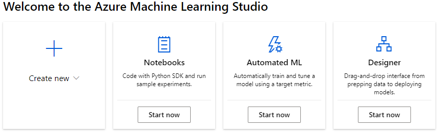
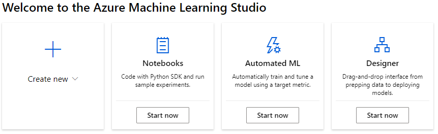
Azure ML studio provides 3 artifacts for conducting machine learning experiments.
Notebooks
Automated ML
Designer
In this article, we will see how we can use notebooks to build a machine learning experiment.
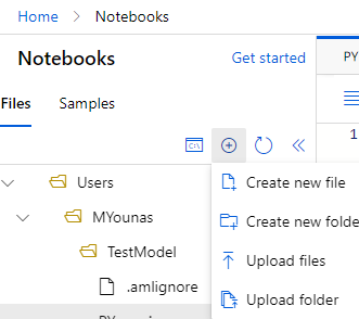
From Azure ML studio, Click on Start now button on the Notebooks (or, alternatively, click on create new -> Notebook)
I have created a new folder TestModel, and a file called main.py from the interface above.
Structure of Azure Experiment:
It’s important to understand the structure of an experiment in azure and the components involved in successfully executing one.
Workspace:
Azure Machine Learning Workspace is the environment which provides all the resources required to run an experiment. For example, if we were to create a word document, then Microsoft Word in this example would be equivalent to a workspace as it provides all the resources.
Experiment:
An Experiment is a group of Runs ( actual instances of experiments). To create a machine learning model, we may have to create experiment runs multiple times. What groups the individual runs together is an experiment.
Run:
A run is an individual instance of an experiment. A run is one single execution of code. We use run to capture output, analyze results and visualize metrics. If we have 5 runs in an experiment. We can compare the same metrics for 5 runs in one experiment to evaluate the best run and work towards anoptimum model.
Environment:
The environment is another important concept in Azure Machine learning. It defines
Python packages
Environment variables
Docker settings
An Environment is exclusive to the workspace it is created in and cannot be used across different workspaces.
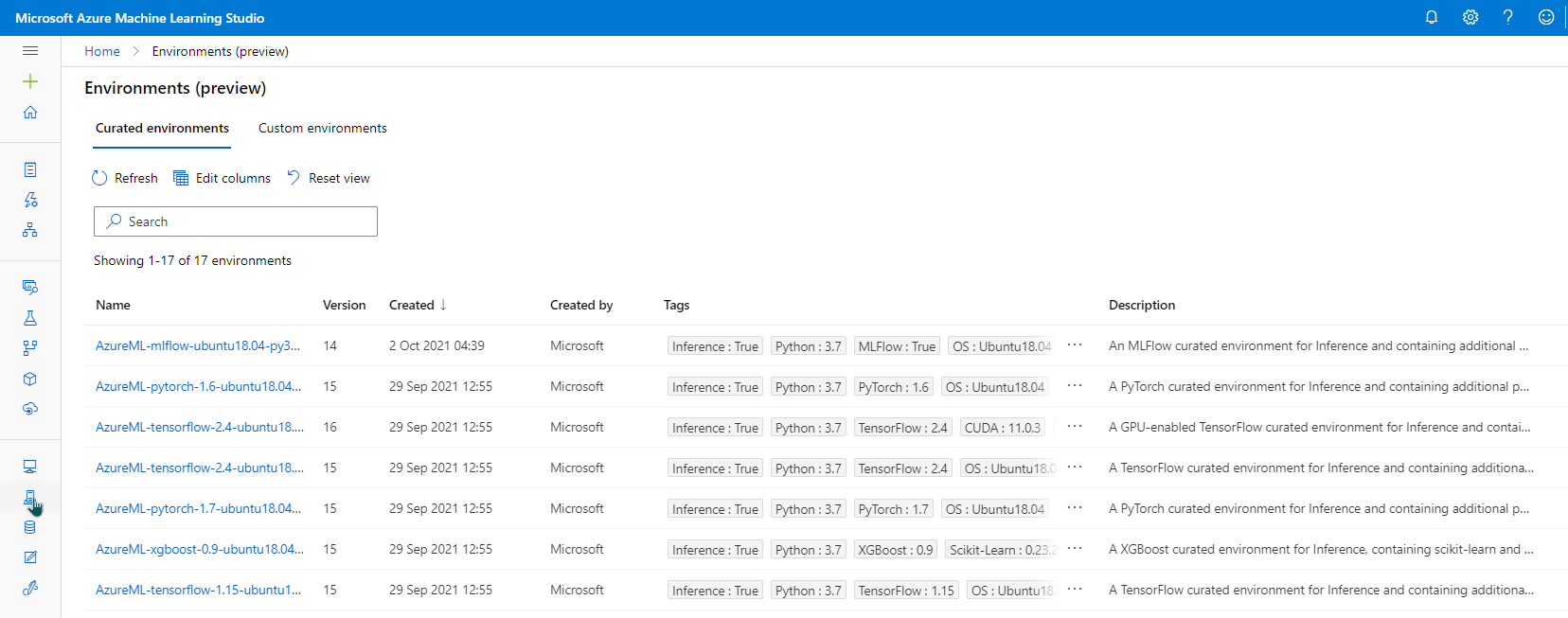
Types of environments:
There are 3 types of environments supported in Azure Machine Learning.
Curated: Provided by Azure, intended to be used as-is. Helpful in getting started.
User-Managed: We( set up the environment and install packages that are required on compute target.
System-Managed: Used when we want Conda to manage Python environment and script dependencies.
We can look at curated and system-managed environments from the environment link in Azure ML Studio.
To create an experiment, we use a control script. The control script decides workspace, experiment, run and some other configuration required to run an experiment.
Creating Control Script
A control script is used to control how and where your machine learning code is run.
Experiment class provides a way to organize multiple runs under a single name.
3
config = ScriptRunConfig(
This function is used to configure how we want our compute to run our script in Azure Machine Learning Workspace
4
run = experiment.submit(config)
This function submits a run. A run is a single execution of your code.
5
am_url= run.get_portal_url()
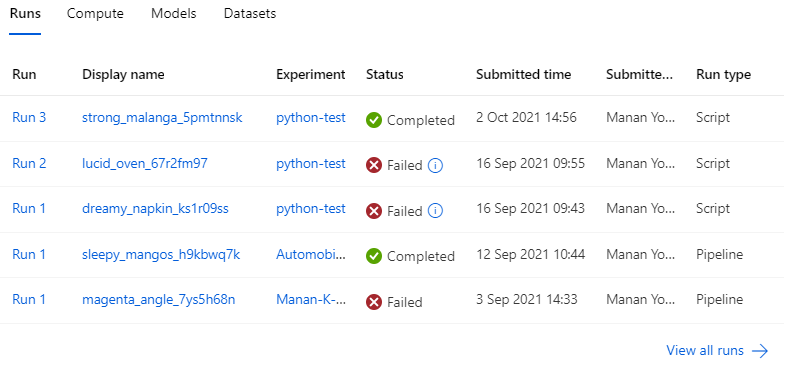
Running the Experiment
Our control script is now capable of instructing Azure Machine Learning workspace to run our experiment from the main.py file. Azure ML studio automatically takes care of creating experiments and run entries in the workspace we specified. To confirm what our code did, we can head back to our Azure ML workspace. It created an Experiment and a run. Azure automatically creates a fancy display name for a run which in our case is strong malanga. My first few runs failed because of some configuration errors. Running it for 3rd time marks a successful run for the experiment python-test.
In the earlier article, we used Azure ML Designer to build a regression model. The final output of the regression model is few metrics which we use to understand how good our regression model is.
There are two steps of interest in evaluating the efficiency of the model. The score model step predicts the price, and evaluate model step finds the difference between prediction and actual price which was already available in the test dataset.
Azure ML Step
Function
Dataset
Train Model
Find mathematical relationship(model) between input data and price
Training dataset
Score Model
Predict prices based on the Training model
Testing dataset.
Added 1 more column of forecasted price.
Evaluate Model
Calculate the difference between prediction and the actual price
Testing data set.
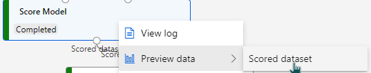
Score Model
Before going to evaluation, it is pertinent to investigate the output of Score Model and what has been scored.
Understanding Scoring
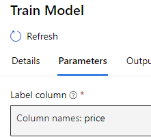
When we were training our model, we selected the Label column as Price.
Training model for label price means in simple terms is :
Using 25 other columns in the data, find what is the best combination of values, which can predict the value of our Label column (price)
Scoring model
Used training model to predict the value of price
Used test dataset and provide a predicted value of price
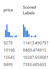
Therefore, after scoring, we will have an extra column added at the end of the scored data set, called Scored Labels. It looks like this in preview
This new column “Scored Labels” is the predicted price. We can use this column to calculate the difference between the actual price which was available in the test data set and how the predicted price (Scored Labels) is
The lower the difference, the better the model is. Hence, we will use the difference as a measure to evaluate the model. There are several metrics which we can use to evaluate the difference.
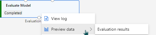
Evaluate Model
We can investigate these metrics by right clicking on Evaluate Model > Preview data > Evaluation results
The following metrics are reported:
Both Mean Absolute Error and Root Mean Square error are averages of errors between actual values and predicted values.
I will take the first two rows of the scored dataset to explain how these metrics evaluate the model.
make
Wheel-base
length
width
….
Price
Predicted price
(Scored Label)
Mitsubishi
96.3
172.4
65.4
…
9279
11413.49
Subaru
97
173.5
65.4
…
10198
8489.47
Absolute Errors
Mean Absolute Error
Evaluates the model by taking the average magnitude of errors in predicted values. A lower value is better
Using the table above, MAE will be calculated as :
Price
Predicted price
(Scored Label)
Error =
Prediction – Price
Magnitude of error
Average of error
9279
11413.49
2,134.49
2,134.49
854.76
10198
8489.47
-1,708.53
1,708.53
854.76 for the above 2 rows is the average error. Let’s assume there was another model whose MAE will be 500.12. If we were comparing two models
Model 1 : 854.76
Model 2 : 500.12
In this case, model 2 will be more efficient than Model 1 as its average absolute error is less.
Root Mean Squared error
RMSE also measures average magnitude of the error. A lower value is better. However, differs from Mean Absolute Error in two ways :
it creates a single value that summarized the error
Errors are squared before they are averaged, hence it gives relatively high weight to large errors. E.g., if we had 2 error values of 2 & 10, squaring them would make them 4 and 100 respectively. This means that larger values get disproportionately large weightage.
This means RMSE should be more useful when large errors are particularly undesirable.
Using the table above, RMSE will be calculated as :
Price
Predicted price
(Scored Label)
Error =
Prediction – Price
Square of Error
Average of Sq. Error
Square root.
9279
11413.49
2,134.49
4,556,047.56
3,737,561.16
10198
8489.47
-1,708.53
2,919,074.76
Relative Errors
To calculate relative error, we first need to calculate the absolute error. Relative error expresses how large the absolute error is compared with the total object we are measuring.
Relative Error = Absolute Error / Known Value
Relative error is expressed as a fraction, or multiplied by 100 to be expressed as a percent.
Relative Squared error
Relative squared error compares absolute error relative to what it would have been if a simple predictor had been used.
This simple predictor is average of actual values.
Example :
In the Automobile price prediction, we have an absolute error of our model which is Total Squared Error.
Instead of using our model to predict the price, if we just take an average of the “price” column. Then find squared error based on this simple average. It will give us a relative benchmark to evaluate our original error with.
Therefore, the relative square error will be :
Relative Squared Error = Total Squared Error / Total Squared Error of simple predictor
Using the two-row example to calculate RSE :
Calculate Sum of Squared based on Simple Predictor of Average
Price
Average of Price
(New Scored Label)
Error =
Prediction – Price
Sum of Squared
9279
9,738.5
459.5
10198
9,738.5
459.5
Mathematically relative squared error, Ei of an individual model i is evaluated by :
Relative Absolute Error
RAE compares a mean error to errors predicted by a trivial or naïve model. A good forecasting model will produce a ratio close to zero. A poor model will produce a ratio greater than 1.
Relative Absolute Error = Total Absolute Error / Total Absolute Error of simple predictor
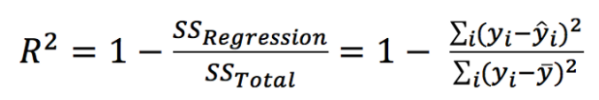
Coefficient of determination
The coefficient of determination represents the proportion of variance for a dependent variable (Prediction) that’s explained by an independent variable (attribute used to predict).
In contrast with co-relation which explains the strength of the relationship between independent and dependent variables, the Coefficient of determination explains to what extent variance of one variable explains the variance of the second variable.
Azure machine learning studio provides an easy-to-use interface for data scientists and developers to build train and productionise machine learning models. Another major benefit it provides is the ease of collaboration and
In this article, we will explore how to solve a machine learning problem with Azure Machine Learning Designer.
Defining the Problem
To solve the problem via Azure ML Studio. We need to do the following steps
Create a Pipeline,
Set pipeline’s compute target.
Importing Data
Transforming Data
Train the Model
Testing the Model
Evaluate the Model
Creating pipeline using ML Designer
Azure machine learning pipelines are workflows of executable steps that enable users to complete Machine Learning workflows. Executable steps in azure pipelines include data import, transformation, feature engineering, model training, model optimisation, deployment etc.
There are 3 ways of creating pipelines in Azure Machine learning Studio
Using Code ( Python SDK )
Using Auto ML
Using ML Designer.
When we login to Azure ML Studio , we see the following options.
Click on Designer (Start Now) to create a new Pipeline.
By default it’s given a name based on today’s date. I have changed it to Automobile Prediction.
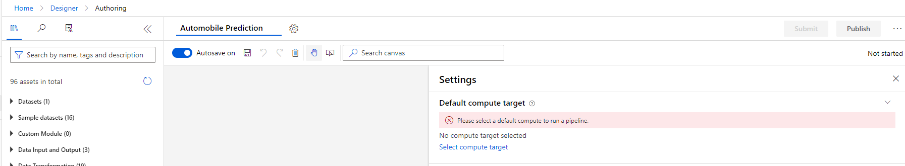
Setting Compute Target
A compute target is an instance of Azure virtual machine which will be used to provide processing power for our pipeline execution.
Default compute target will be used for entire pipeline, we can also use separate compute targets for individual steps of execution.
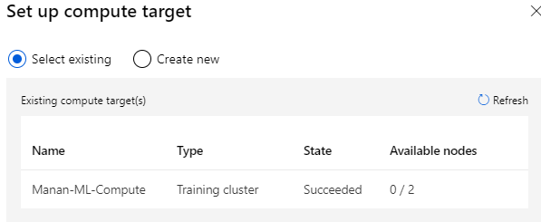
I created a compute instance earlier, so I can select existing
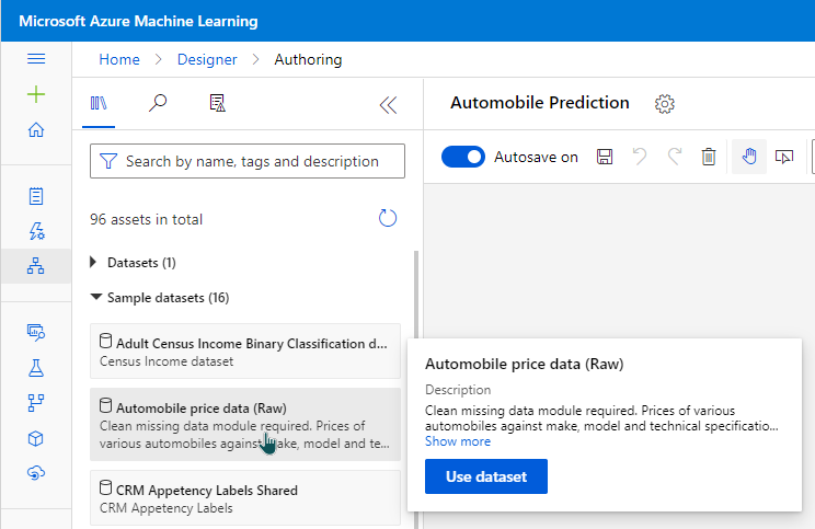
Importing Data
We can import the data from several sources. For this article, I will use sample datasets provided by Azure.
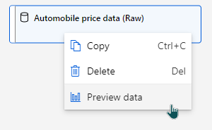
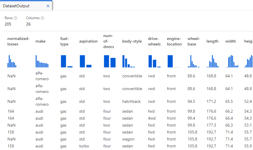
To explore what is in the data set, we can click on the data set and go to preview data.
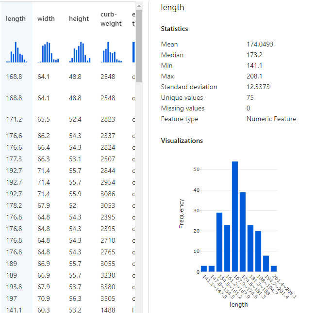
This provides us a sneak-preview of what’s included in the data. E.g. there are 205 rows, 26 columns. Clicking on each column provides key statistics about data in that specific column. E.g. If I click on length column, I get a histogram showing the frequency of length values and various other statistics about it.
Transform Data
The data preview feature is helpful in understanding the columns and transforming data for any characteristics necessary to run our model.
Exclude a column
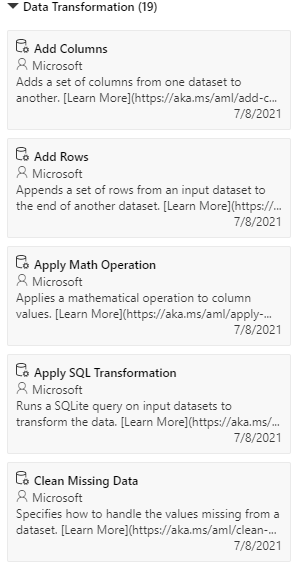
The data transformation section on left side menu provides several commonly used data transformation operations.
I want to remove the column normalized-losses
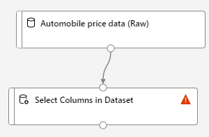
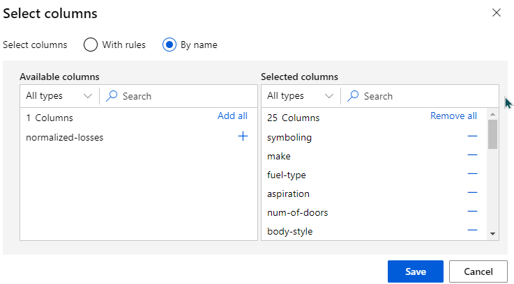
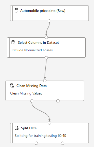
So, I can drag and drop “Select Columns in Dataset”
When I go to the details of “Select Columns in Dataset” , I can then select all columns other than normalized losses
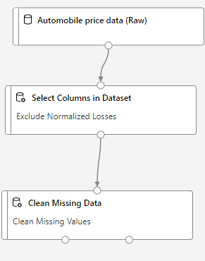
Clean Missing Data
After removing the normalized-losses columns, our data still has empty values. To clean the missing data. I can use Clean Missing Data module from left side menu. So that our worspace looks like
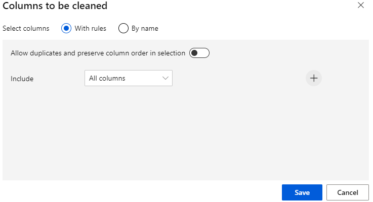
Going into details of Cleaning missing data, I can select Alll columns.
Training the Model
I want to divide my dataset rows into
Training rows (training dataset)
Testing rows (testing dataset)
I can use Split Data Module from left side menu, so that my pipeline will now look like :
The Split Data module has 2 outputs. The left outputwill connect to Train Model and Right output will connect to Test Data.
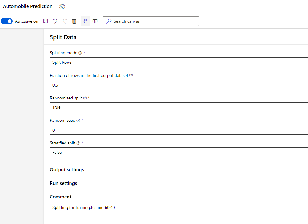
In the details of Split Data module, I can choose the ratio with which I want to split the data across training and testing.
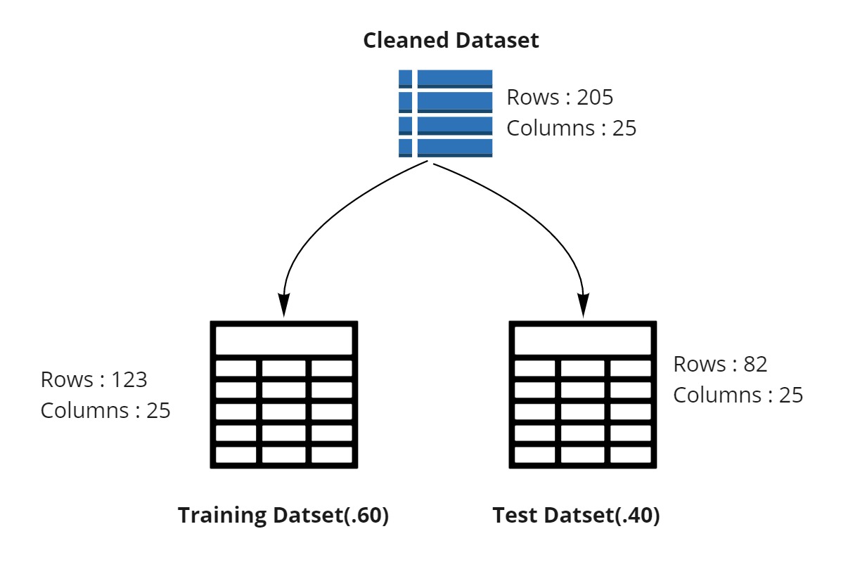
In summary, we cleaned the dataset and then divided it into two separate one as shown in the image below.
Training the Model
To train any model, we need to have.
The model
The data on which model is to be trained.
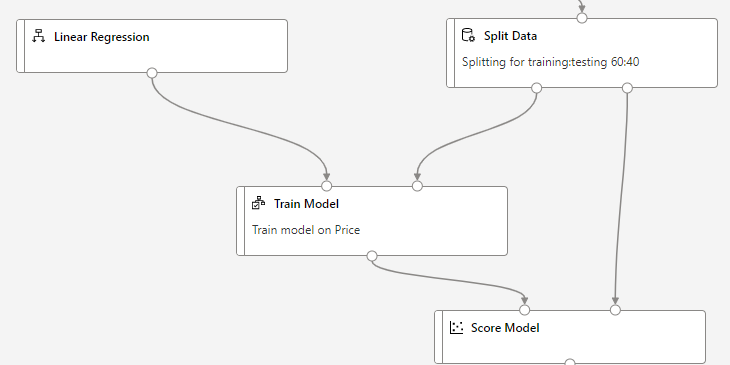
In our case, we want to predict automobile prices using Linear Regression Model. The training data for Linear Regression Model is the one which we have split from our overall data.
Therefore, we can train our model by combination of Linear Regression module and Train Model module from left side menu.
The Train Model module requires a label to train the model for. A label in this case is independent variable? with the help of which we can find the dependent variable.
[From y = mx + c , a label is X ]
Testing the Model
In Split Data step above, we used only 60 % of our data for training the model. We left remaining 40% of the data for testing. We can setup the testing now by using Score Model module.
Score Model module will need two input.
What needs to be tested (output of our trained model)
With what to test (test data from split)
This will look like:
Evaluating the Model
Now we want to see how our model scored when compared against the test dataset. We can use Evaluate Model module and connect Score Model module to it.
This will finish our pipeline creation. We now need to submit it.
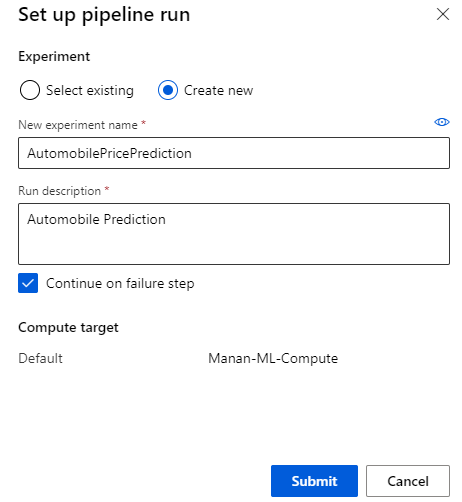
Pipeline Submission
Pipeline submission will create an experiment name and compute target.
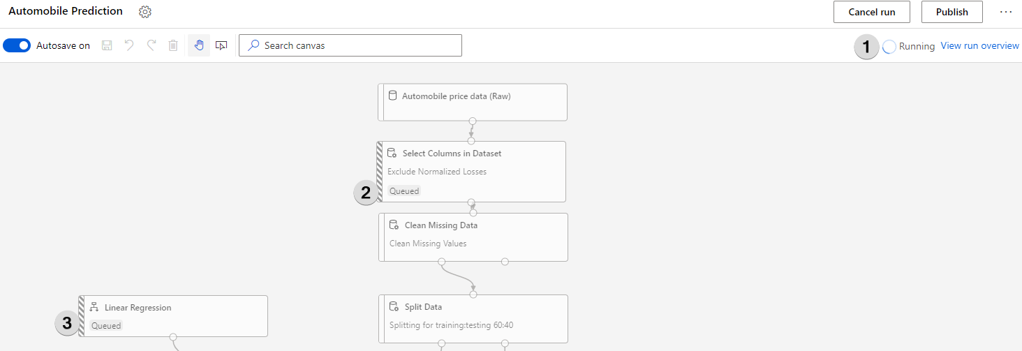
Understanding the Predictions
Azure ML takes a bit of time especially if the experiment is run for the first time. You can view the progress by looking at the “Running” status (1) or by looking at what’s the status of each individual module ( 2, 3).
Once the model finishes it run, right-click on Score Model and select Visualize > Scored dataset
In the Scored Labels column, you can see the predicted prices.
Understanding Models efficiency
We can use Evaluate Model to see the efficiency of the trained mode.
Right click Evaluate Model -> Visualize -> Evaluation Results