MapReduce is a fundamental algorithmic model used in distributed computing to process and generate large datasets efficiently. It was popularized by Google and later adopted by the open-source community through Hadoop. The model simplifies parallel processing by dividing work into map and reduce tasks, making it easier to scale across a cluster of machines. Whether you’re working in big data or learning Apache Spark, understanding MapReduce helps in building a strong foundation for distributed data processing.
What Is MapReduce?
MapReduce is all about breaking a massive job into smaller tasks so they can run in parallel.
- Map: Each worker reads a bit of the data and tags it with a key.
- Reduce: Another worker collects all the items with the same tag and processes them.
That’s it. Simple structure, massive scale.
Why Was MapReduce Needed?
MapReduce emerged when traditional data processing systems couldn’t handle the explosive growth of data in the early 2000s, requiring a new paradigm that could scale horizontally across thousands of commodity machines. Given below is a brief rundown of what problems existed for handling Big Data and how MapReduce solved it.
| Problem | MapReduce Solution |
| Data Volume Explosion: Single machines couldn’t handle terabytes/petabytes of data | Automatic data splitting and distributed processing across multiple machines |
| Network failures and system crashes | Built-in fault tolerance with automatic retry mechanisms and task redistribution |
| Complex load balancing requirements | Automated task distribution and workload management across nodes |
| Data consistency issues in distributed systems | Structured programming model ensuring consistent data processing across nodes |
| Manual recovery processes after failures | Automatic failure detection and recovery without manual intervention |
| Difficult parallel programming requirements | Simple programming model with just Map and Reduce functions |
| Poor code reusability in distributed systems | Standardized framework allowing easy code reuse across applications |
| Complex testing of distributed applications | Simplified testing due to the standardized programming model |
| Expensive vertical scaling (adding more CPU/RAM) | Cost-effective horizontal scaling by adding more commodity machines |
| Data transfer bottlenecks | Data locality optimization by moving computation to data |
Schema-on-Read:
Schema-on-read is backbone of MapReduce. It means you don’t need to structure your data before storing it. Think of it like this:
- Your input data can be messy – log files, CSVs, or JSON – MapReduce doesn’t care
- Mappers read and interpret the data on the fly, pulling out just the pieces they need
- If some records are broken or formatted differently, the mapper can skip them and keep going
Example: Let’s say you’re processing server logs. Some might have IP addresses, others might not. Some might include user agents, others might be missing them. With schema-on-read, your mapper just grabs what it can find and moves on – no need to clean everything up first.
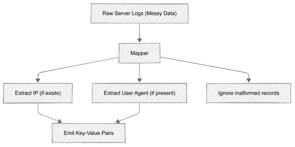
MapReduce doesn’t care what your data looks like until it reads it. That’s schema-on-read. Store raw files however you want, and worry about structure only when you process them.
How MapReduce Works in Hadoop
Let’s walk through a realistic example. Imagine a CSV file with employee info and we want to count the number of employees in each department :
101, Alice, HR
102, Bob, IT
103, Clara, HR
104, Dave, Finance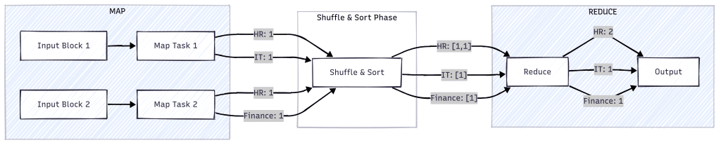
Step 1: Input Split and Mapping
First, Hadoop splits the input file into blocks—say, 128MB each. Why? So they can be processed in parallel across multiple machines. That’s how Hadoop scales.
Each Map Task reads lines from its assigned block. In our case, each line represents an employee record, like this:
101, Alice, HR
What do we extract from this? It depends on our goal. Since we’re counting people per department, we group by department. That’s why we emit:
("HR", 1)We don’t emit ("Alice", 1) because we’re counting departments, not individuals. This key-value pair structure prepares us perfectly for the reduce phase.
Step 2: Shuffle and Sort
These key-value pairs then move into the shuffle phase, where they’re grouped by key:
("HR", [1, 1])

("IT", [1])

("Finance", [1])
Step 3: Reduce
Each reducer receives one of these groups and sums the values:
("HR", 2)

("IT", 1)

("Finance", 1)
The final output shows the headcount per department.
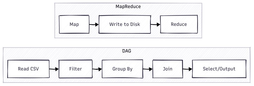
MapReduce Today: The Evolution to DAG-Based Processing
While MapReduce revolutionized distributed computing, its rigid two-stage model had limitations. Each operation required writing to disk between stages, creating performance bottlenecks. Apache Spark introduce the concept of DAG ( Directed Acyclic Graph)
The DAG model represents a fundamental shift in how distributed computations are planned and executed:
- Flexible Pipeline Design: Instead of forcing everything into map and reduce steps, Spark creates a graph of operations that can have any number of stages
- Memory-First Architecture: Data stays in memory between operations whenever possible, dramatically reducing I/O overhead
- Intelligent Optimization: The DAG scheduler can analyze the entire computation graph and optimize it before execution
- Lazy Evaluation: Operations are planned but not executed until necessary, allowing for better optimization
This evolution meant that while MapReduce jobs had to be explicitly structured as a sequence of separate map and reduce operations, Spark could automatically determine the most efficient way to execute a series of transformations. This made programs both easier to write and significantly faster to execute.
MapReduce vs. DAG: Comparison
Here’s a high level overview of how DAG in spark differs from MapReduce
| Feature | MapReduce | DAG (Spark) |
| Processing Stages | Fixed two stages (Map and Reduce) | Multiple flexible stages based on operation needs |
| Execution Flow | Linear flow with mandatory disk writes between stages | Optimized flow with in-memory operations between stages |
| Job Complexity | Multiple jobs needed for complex operations | Single job can handle complex multi-stage operations |
| Performance | Slower due to disk I/O between stages | Faster due to in-memory processing and stage optimization |
Key Advantages of DAG over MapReduce:
- DAGs can optimize the execution plan by combining and reordering operations
- Simple operations can complete in a single stage instead of requiring both map and reduce
- Complex operations don’t need to be broken into separate MapReduce jobs
- In-memory data sharing between stages improves performance significantly
This evolution from MapReduce to DAG-based processing represents a significant advancement in distributed computing, enabling more efficient and flexible data processing pipelines. For example you could use a much complex chaining of operations using a single line of code in multi-stage Dag as given below:
// Example of a complex operation in Spark creating a multi-stage DAG
val result = data.filter(...)
               .groupBy(...)
               .aggregate(...)
               .join(otherData)
               .select(...)
Understanding the Employee count Code Example
The employee count by department example we discussed above can be written in spark by using these 2 lines.
val df = spark.read.option("header", "true").csv("people.csv")
df.groupBy("department").count().show()
This code performs a simple but common data analysis task: counting employees in each department from a CSV file. Here’s what each part does:
- Line 1: Reads a CSV file containing employee data, telling Spark that the file has headers
- Line 2: Groups the data by department and counts how many employees are in each group
Let’s break down this Spark code to understand how it implements MapReduce concepts and leverages DAG advantages:
1. Schema-on-Read :
- The line
spark.read.option("header", "true").csv("people.csv")demonstrates schema-on-read – Spark only interprets the CSV structure when reading, not before. - It automatically detects column types and handles messy data without requiring pre-defined schemas.
2. Hidden Map Phase with DAG Optimization:
- When
groupBy("department")runs, Spark creates an optimized DAG of tasks instead of a rigid map-reduce pattern. - Each partition is processed efficiently with the ability to combine operations in a single stage when possible.
3. Improved Shuffle and Sort:
- The
groupByoperation triggers a shuffle, but unlike MapReduce, data stays in memory between stages. - DAG enables Spark to optimize the shuffle pattern and minimize data movement across the cluster.
4. Enhanced Reduce Phase:
- The
count()operation is executed as part of the DAG, potentially combining with other operations. - Unlike MapReduce’s mandatory disk writes between stages, Spark keeps intermediate results in memory.
5. DAG Benefits in Action:
- The entire operation is treated as a single job with multiple stages, not separate MapReduce jobs.
- Spark’s DAG optimizer can reorder and combine operations for better performance.
While the code looks simpler, its more than syntax simplification – the DAG-based execution model provides fundamental performance improvements over traditional MapReduce while maintaining the same logical pattern.
Code Comparison: Spark vs Hadoop MapReduce
Let’s compare how the same department counting task would be implemented in both Spark and traditional Hadoop MapReduce:
1. Reading Data
Spark:
val df = spark.read.option("header", "true").csv("people.csv")
Hadoop MapReduce:
public class EmployeeMapper extends Mapper<LongWritable, Text, Text, IntWritable> {
    private final static IntWritable one = new IntWritable(1);
    private Text department = new Text();

    public void map(LongWritable key, Text value, Context context) throws IOException, InterruptedException {
        String[] fields = value.toString().split(",");
        department.set(fields[2].trim());  // department is third column
        context.write(department, one);
    }
}
2. Processing/Grouping
Spark:
df.groupBy("department").count()
Hadoop MapReduce:
public class DepartmentReducer extends Reducer<Text, IntWritable, Text, IntWritable> {
    public void reduce(Text key, Iterable<IntWritable> values, Context context) throws IOException, InterruptedException {
        int sum = 0;
        for (IntWritable val : values) {
            sum += val.get();
        }
        context.write(key, new IntWritable(sum));
    }
}
3. Job Configuration and Execution
Spark:
// Just execute the transformation
df.groupBy("department").count().show()
Hadoop MapReduce:
public class DepartmentCount {
    public static void main(String[] args) throws Exception {
        Job job = Job.getInstance(new Configuration(), "department count");
        job.setJarByClass(DepartmentCount.class);

        job.setMapperClass(EmployeeMapper.class);
        job.setReducerClass(DepartmentReducer.class);

        job.setOutputKeyClass(Text.class);
        job.setOutputValueClass(IntWritable.class);

        FileInputFormat.addInputPath(job, new Path(args[0]));
        FileOutputFormat.setOutputPath(job, new Path(args[1]));

        System.exit(job.waitForCompletion(true) ? 0 : 1);
    }
}
Key Differences:
- Spark requires significantly less boilerplate code
- Hadoop MapReduce needs explicit type declarations and separate Mapper/Reducer classes
- Spark handles data types and conversions automatically
- Hadoop MapReduce requires manual serialization/deserialization of data types
- Spark’s fluent API makes the data processing pipeline more readable and maintainable
Performance Implications:
- Spark keeps intermediate results in memory between operations
- Hadoop MapReduce writes to disk between map and reduce phases
- Spark’s DAG optimizer can combine operations for better efficiency
- Hadoop MapReduce follows a strict two-stage execution model