What is Regression Analysis
Regression analysis is a process to find a relationship between two or more variables.
A variable can represent data from any word, event, occurrence, phenomenon, etc.
For example, say we want to find whether there’s any relationship between cold weather and coffee sales in Melbourne. First variable is cold weather, the second variable is increase in coffee sales.
We can use Regression Analysis to find out
- Whether there’s any relationship between cold weather and coffee sales.
- What is the extent of this relationship? Does cold weather double coffee sales or half it?
Objectives of Regression Analysis
The primary objective of regression analysis is to:
- Determine the relationship between two variables.
- Predict future results based on existing knowledge.
Digital Analytics Use Cases of Regression Analysis
Regression analysis is frequently used in web analytics, digital marketing analytics and other machine learning algorithms. Few examples would be:
- Understanding the impact of Digital marketing channels on Sales. For example, If you are using digital marketing and TV ads. You can establish a relationship between your online & offline channels on your net sales.
- If your website offers paid services, you can use regression analysis to predict whether a customer is likely to leave your paid service. Hence you can take proactive action to stop the customer from churning.
Methods of Regression Analysis
There are several methods used for regression depending on the use case. For example, linear regression, logistic regression, and mixed regression.
Linear Regression
We will focus on linear regression as its simplest to understand
1.Data Representation on Graph
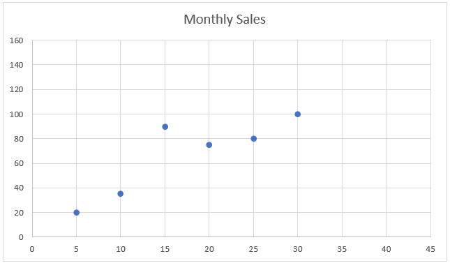
Let’s say we want to find out a relationship between advertising cost and online sales. We have data for 5 campaigns.
| Digital Ad Dollars (Million) | Monthly E-commerce sale (Million) |
| 5 | 20 |
| 20 | 75 |
| 10 | 46 |
| 25 | 80 |
| 30 | 100 |
To get a visual understanding of our data. Let’s put them on a scatter plot
(A scatter is a graphical way of representing the relationship between two variables)

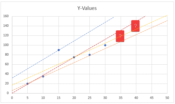
Our task is to establish a relationship so that we can use that relationship to predict future sales. In our example, we want to find out what would be our sale if we spend 40 million dollars or 45 million dollars.
| Digital Ad Dollars (Million) | Monthly E-commerce sale (Million) |
| 35 | ? |
| 40 | ? |

2.Assuming straight lines
Let’s assume that there’s a straight line running through the graph that predicts the future value with 100% accuracy. If we could predict the data accurately, the values for X-axis 35 and 40 will land precisely on our perfect assumption line. However, that’s an unknown.
If we could visually draw assumption lines to “predict” relationship, then we can theoretically draw unlimited lines, one of them would be perfect. We cannot know which one.
Linear regression forecasts the value of unknown data points ( in our example, 35 & 40) by finding the best fit line through the points. The best-fitting line is called a regression line.

3.Best Fit line – Regression line
A best-fit line should minimize the error between values forecasted by it and the actual ( unknown ) values.
Different methods are available for finding the best fit line. Few of the methods are
- Generalized method of moments ( GMM)
- Maximum Likelihood estimation ( ML)
- Ordinary Least Square method ( OLS)
Most used method is ordinary least square method.
Ordinary Least Square method
Least square method was officially discovered & published by Adrien-Marie in 1805. Ordinary least square method works by minimizing the sum of squares of the known ( observed) values and those predicted by the linear function.
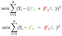
If we could plot n random lines through the points and calculate the sum of residuals ( distance from observed value to the value on our assumed line), each line will have multiple error values( one for each data point) . Summing up those values and then squaring them will give us a single number. Let’s call it sum of squares. If we drew 10 lines, we will have 10 different sum of squares. Our task is to find the value with the least sum of squares.
Mathematically sum of squares errors can be written as

Where
![]() : is the actual value
: is the actual value
![]() : is the estimated (or predicted) Y value
: is the estimated (or predicted) Y value
The predicted value can be calculated using a simple line equation
![]()
Replacing the value of estimated ( or predicted ) Y value in the sum of square error equation.

From here, we can use calculus to differentiate this equation with respect to the first regression coefficient and set it to zero, then differentiate with respect to other regression coefficient and set it to zero, thus deriving sample regression function.
SRF (Sample Regression Function) :
![]()
Where
![]() : is the slope and can also be written as.
: is the slope and can also be written as.

![]() : is the intercept and can also be written as
: is the intercept and can also be written as
![]()
